Amazon SageMaker 中 GPU 对计算加速效果的分析与验证

背景介绍

Amazon SageMaker 是一项完全托管的服务，可以帮助开发人员和数据科学家快速构建、训练和部署机器学习 (ML) 模型。然而用户在Amazon SageMaker的日常使用中，常常会有如下疑问：“我的SageMaker 中GPU实例里面真的有GPU吗？”,“我的SageMaker 中的GPU真的起到加速作用了吗？”，”为什么我的SageMaker 中GPU实例的运算速度并没有比CPU实例中的运算速度更快？”。

本文主要介绍如何查看实例中GPU的运行状态，如何测试并对比CPU与GPU的性能，如何在SageMaker Studio中分别运用CPU和GPU进行神经网络的训练。希望通过这篇文章，您可以对SageMaker中GPU的加速能力有更全面的体会。

本文的相关代码可以在GitHub仓库中获得。

确定GPU的个数与运行状态

本文中的代码将在SageMaker Notebook中运行，首先新建一个Notebook（新手教程），并选取一个具有GPU的Kernel，本文中选取的是ml.p3.8xlarge实例，并选择conda_tensorflow2_p36 Kernel。根据该实例的参数可以得知，其配有4个GPU。接下来我们将通过指令查看具体的GPU型号，以及其运行状态。在Notebook中运行：

tf.config.list_physical_devices("GPU")

我们可以看到具体的GPU型号的输出：

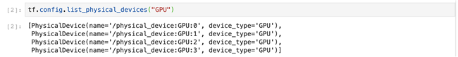
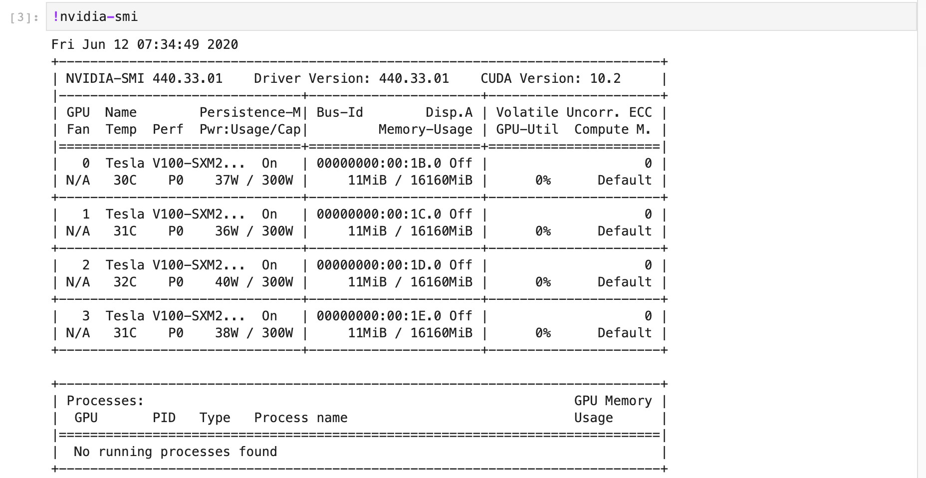
注意，GPU的编号从0开始，图中的输出表示该实例拥有四个GPU。接下来我们将继续查看该GPU的型号以及运行状态，在Notebook中运行：

!nvidia-smi

我们可以看到如截图所示，其中不同字段的具体含义如下：

Fan：风扇转速（0%–100%），N/A表示没有风扇

Temp：GPU温度

Perf：性能状态，从P0（最大性能）到P12（最小性能）

Pwr：GPU功耗

Persistence-M：持续模式的状态

Bus-Id： GPU总线，格式为：domain:bus:device.function

Disp.A： Display Active，表示GPU的显示是否初始化

Memory-Usage：显存使用率

Volatile GPU-Util：GPU使用率

ECC：是否开启错误检查和纠正技术，0/DISABLED, 1/ENABLED

Compute M.：计算模式，0/DEFAULT,1/EXCLUSIVE_PROCESS,2/PROHIBITED

CPU与GPU的性能大比拼

在确定SageMaker Studio 的Notebook实例的确配有GPU实例后，我们将通过具体实验来测试GPU的计算性能，并与CPU在相同场景下的计算性能进行比较。

矩阵运算场景

我们设计一个简单的计算场景：随机生成一个维度x = 10000的矩阵，将该矩阵与其转置点乘，然后再求和。让我们在Notebook中输入如下代码，对GPU的计算进行测速，这里我们指定使用编号为0的GPU进行运算：

#!/usr/bin/env python
# -*- coding:utf-8 -*-
import sys
import tensorflow as tf
from datetime import datetime

shape = (10000, 10000)

device_name = "/gpu:0"
with tf.device(device_name):
    random_matrix = tf.random.uniform(shape=shape, minval=0, maxval=1)
    dot_operation = tf.matmul(random_matrix, tf.transpose(random_matrix))
    sum_operation = tf.reduce_sum(dot_operation)
 
startTime = datetime.now()
with tf.compat.v1.Session(config=tf.compat.v1.ConfigProto(log_device_placement=True)) as session:
        result = session.run(sum_operation)
        
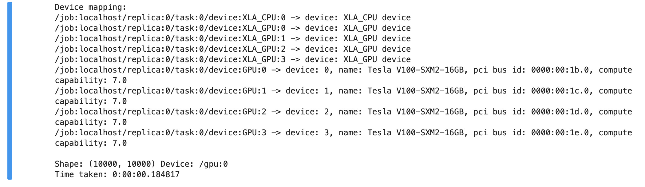
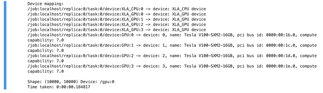
print("Shape:", shape, "Device:", device_name)
print("Time taken:", datetime.now() - startTime)

可以看到计算结果如下，GPU耗时0.184817秒：

随后在Notebook中输入下述CPU性能测试代码：

device_name = "/cpu:0"
with tf.device(device_name):
    random_matrix = tf.random.uniform(shape=shape, minval=0, maxval=1)
    dot_operation = tf.matmul(random_matrix, tf.transpose(random_matrix))
    sum_operation = tf.reduce_sum(dot_operation)
 
startTime = datetime.now()
with tf.compat.v1.Session(config=tf.compat.v1.ConfigProto(log_device_placement=True)) as session:
        result = session.run(sum_operation)
        
print("Shape:", shape, "Device:", device_name)
print("Time taken:", datetime.now() - startTime)

可以看到计算结果如下，CPU耗时2.587753秒：

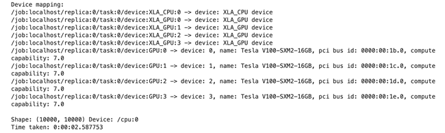
综上，在矩阵维度为10000时，GPU的速度约为CPU的14倍。

那么，是否任何情况下GPU的性能都优于CPU呢？

带着这个疑问，我们令矩阵的维度为变量，分别从10增长到20000，观测计算时间的变化。让我们在Notebook中输入下述代码：

shape_index = [10, 50, 100, 200, 300, 400, 500, 600, 700, 800, 900, 1000, 2000, 3000, 4000, 5000, 6000, 7000, 8000, 9000, 10000, 11000, 12000, 13000, 14000, 15000, 16000, 17000,18000, 19000, 20000]
gpu_time = []
cpu_time = []

for i in shape_index:
    print("shape is %d"%i)
    shape = (i, i)
    
    device_name = "/gpu:0"
    with tf.device(device_name):
        random_matrix = tf.random.uniform(shape=shape, minval=0, maxval=1)
        dot_operation = tf.matmul(random_matrix, tf.transpose(random_matrix))
        sum_operation = tf.reduce_sum(dot_operation)

    startTime = datetime.now()
    with tf.compat.v1.Session(config=tf.compat.v1.ConfigProto(log_device_placement=True)) as session:
            result = session.run(sum_operation)
    
    gpu_time.append((datetime.now() - startTime).total_seconds())
    
    device_name = "/cpu:0"
    with tf.device(device_name):
        random_matrix = tf.random.uniform(shape=shape, minval=0, maxval=1)
        dot_operation = tf.matmul(random_matrix, tf.transpose(random_matrix))
        sum_operation = tf.reduce_sum(dot_operation)

    startTime = datetime.now()
    with tf.compat.v1.Session(config=tf.compat.v1.ConfigProto(log_device_placement=True)) as session:
            result = session.run(sum_operation)
    
    cpu_time.append((datetime.now() - startTime).total_seconds())

运行结束后，我们运用下述可视化代码绘制出计算时间曲线：

%matplotlib inline
import matplotlib.pyplot as plt    
import numpy as np
fig, ax = plt.subplots(nrows=1, ncols=2, figsize=(15,10))
ax[0].plot(shape_index, gpu_time)
ax[0].plot(shape_index, cpu_time)
ax[0].set_xlabel("shape")
ax[0].set_ylabel("cost_time / sec") 
ax[0].set_title("GPU & CPU cost time")

print(cpu_time)
print(gpu_time)
multiple = np.array(cpu_time) / np.array(gpu_time)
ax[1].plot(shape_index, multiple)
ax[1].set_xlabel("shape")
ax[1].set_ylabel("cpu/gpu") 
ax[1].set_title("CPU Time / GPU Time")

plt.show()

结果将如下图所示：

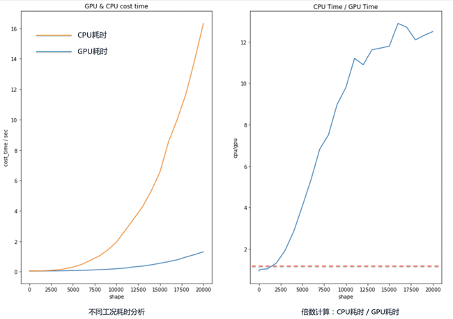
分析上图可知，随着矩阵维度的增加，GPU的优势呈指数上升；同时我们可以发现，在矩阵维度较低时，CPU的性能可能会更好。

神经网络实测场景

通过上述在简单矩阵运算场景下的测试，我们对GPU的性能有了初步的认识。那么接下来将通过完成“MNIST手写数字识别”任务，再次体会GPU性能的优势。

让我们在Notebook中输入下述代码：

import tensorflow as tf
from datetime import datetime

mnist = tf.keras.datasets.mnist
(x_train, y_train), (x_test, y_test) = mnist.load_data()
x_train, x_test = x_train / 255.0, x_test / 255.0


startTime = datetime.now()
with tf.device('/gpu:0'):
    model = tf.keras.models.Sequential([
      tf.keras.layers.Flatten(input_shape=(28, 28)),
      tf.keras.layers.Dense(1000, activation='relu'),
      tf.keras.layers.Dropout(0.2),
      tf.keras.layers.Dense(1000, activation='relu'),
      tf.keras.layers.Dropout(0.2),
      tf.keras.layers.Dense(1000, activation='relu'),
      tf.keras.layers.Dropout(0.2),
      tf.keras.layers.Dense(10, activation='softmax')
    ])

    model.compile(optimizer='adam',
                  loss='sparse_categorical_crossentropy',
                  metrics=['accuracy'])
    
    model.fit(x_train, y_train, epochs=5)
    model.evaluate(x_test, y_test)
gpu_cost_time = datetime.now() - startTime


startTime = datetime.now()
with tf.device('/cpu:0'):
    model = tf.keras.models.Sequential([
      tf.keras.layers.Flatten(input_shape=(28, 28)),
      tf.keras.layers.Dense(1000, activation='relu'),
      tf.keras.layers.Dropout(0.2),
      tf.keras.layers.Dense(1000, activation='relu'),
      tf.keras.layers.Dropout(0.2),
      tf.keras.layers.Dense(1000, activation='relu'),
      tf.keras.layers.Dropout(0.2),
      tf.keras.layers.Dense(10, activation='softmax')
    ])
    model.compile(optimizer='adam',
                  loss='sparse_categorical_crossentropy',
                  metrics=['accuracy'])
    model.fit(x_train, y_train, epochs=5)
    model.evaluate(x_test, y_test)
cpu_cost_time = datetime.now() – startTime
print('GPU Cost Time：%s, CPU Cost Time：%s' % (str(gpu_cost_time), str(cpu_cost_time)))

计算输出如下图所示：

训练结果为：GPU耗时21秒，CPU耗时1分06秒。

我们可以看到，GPU完成相同任务的训练的时间，约为CPU的三分之一。同时这个差距将随着网络结构的复杂而增加。

总结

在这篇博客文章中，您学到了如何查看实例中GPU的运行状态，如何测试并对比CPU与GPU的性能，以及如何在SageMaker Studio中分别运用CPU和GPU进行神经网络的训练。我期待收到您的反馈意见和建议, 想要了解更多内容您可以关注AWS 微博或者微信。

亚马逊AWS官方博客