Build, train, deploy, and monitor a machine learning model
with Amazon SageMaker Studio
Amazon SageMaker Studio is the first fully integrated development environment (IDE) for machine learning that provides a single, web-based visual interface to perform all the steps for ML development.
In this tutorial, you use Amazon SageMaker Studio to build, train, deploy, and monitor an XGBoost model. You cover the entire machine learning (ML) workflow from feature engineering and model training to batch and live deployments for ML models.
In this tutorial, you learn how to:
- Set up the Amazon SageMaker Studio Control Panel
- Download a public dataset using an Amazon SageMaker Studio Notebook and upload it to Amazon S3
- Create an Amazon SageMaker Experiment to track and manage training and processing jobs
- Run an Amazon SageMaker Processing job to generate features from raw data
- Train a model using the built-in XGBoost algorithm
- Test the model performance on the test dataset using Amazon SageMaker Batch Transform
- Deploy the model as an endpoint, and set up a Monitoring job to monitor the model endpoint in production for data drift.
- Visualize results and monitor the model using SageMaker Model Monitor to determine any differences between the training dataset and the deployed model.
The model will be trained on the UCI Credit Card Default dataset that contains information on customer demographics, payment history, and billing history.
| About this Tutorial | |
|---|---|
| Time | 1 hour |
| Cost | Less than $10 |
| Use Case | Machine Learning |
| Products | Amazon SageMaker |
| Audience | Developer, Data Scientist |
| Level | Intermediate |
| Last Updated | February 25, 2021 |
Step 1. Create an AWS Account
The resources created and used in this tutorial are AWS Free Tier eligible. The cost of this workshop is less than $10.
Already have an account? Sign-in
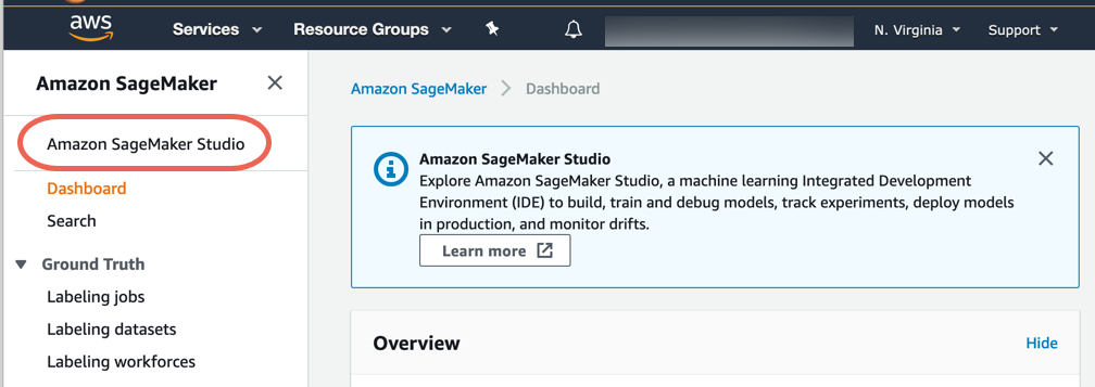
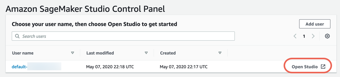
Step 2. Create your Amazon SageMaker Studio Control Panel
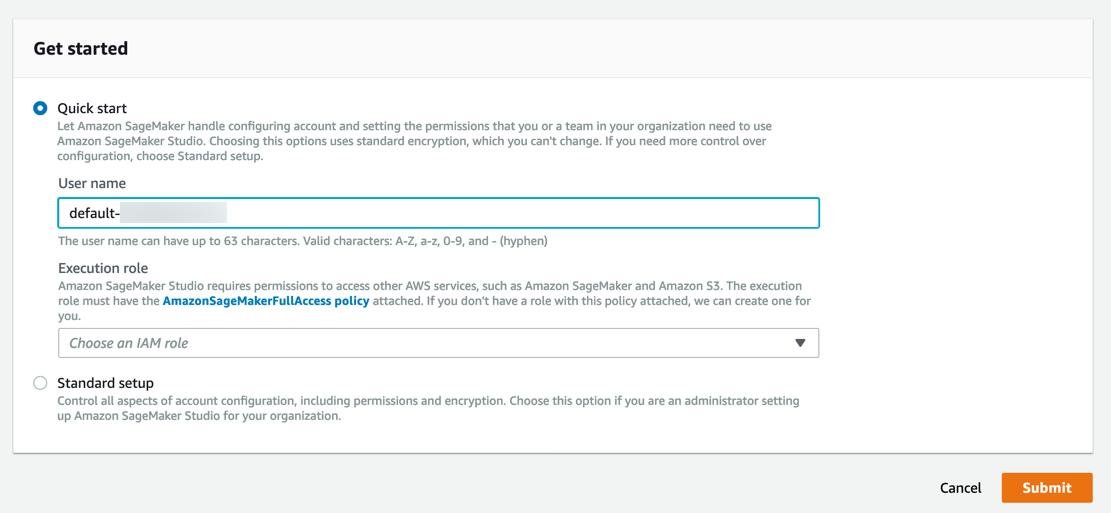
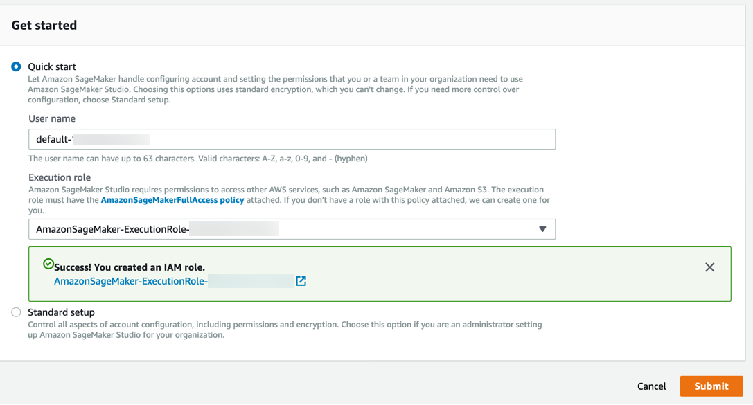
Complete the following steps to onboard to Amazon SageMaker Studio and set up your Amazon SageMaker Studio Control Panel.
Note: For more information, see Get Started with Amazon SageMaker Studio in the Amazon SageMaker documentation.
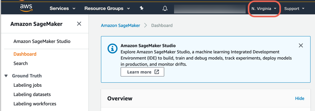
a. Sign in to the Amazon SageMaker console.
Note: In the top right corner, make sure to select an AWS Region where SageMaker Studio is available. For a list of Regions, see Onboard to Amazon SageMaker Studio.
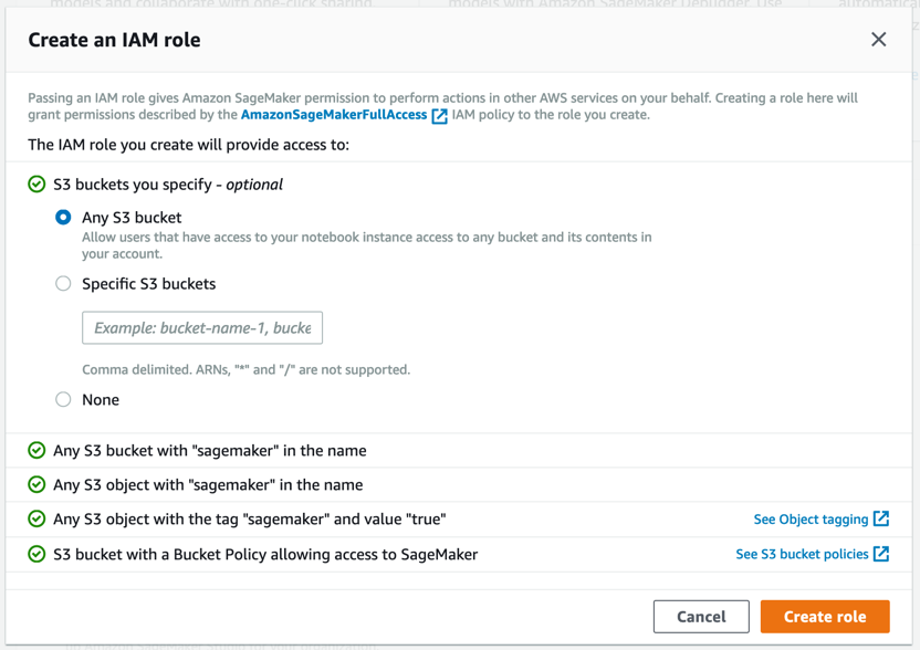
Amazon SageMaker creates a role with the required permissions and assigns it to your instance.
Step 3. Download the dataset
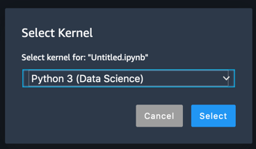
Amazon SageMaker Studio notebooks are one-click Jupyter notebooks that contain everything you need to build and test your training scripts. SageMaker Studio also includes experiment tracking and visualization so that it’s easy to manage your entire machine learning workflow in one place.
Complete the following steps to create a SageMaker Notebook, download the dataset, and then upload the dataset to Amazon S3.
Note: For more information, see Use Amazon SageMaker Studio Notebooks in the Amazon SageMaker documentation.
import boto3
import sagemaker
from sagemaker import get_execution_role
import sys
import IPython

if int(sagemaker.__version__.split('.')[0]) == 2:
    print("Installing previous SageMaker Version and restarting the kernel")
    !{sys.executable} -m pip install sagemaker==1.72.0
    IPython.Application.instance().kernel.do_shutdown(True)

else:
    print("Version is good")


role = get_execution_role()
sess = sagemaker.Session()
region = boto3.session.Session().region_name
print("Region = {}".format(region))
sm = boto3.Session().client('sagemaker')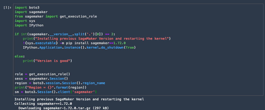
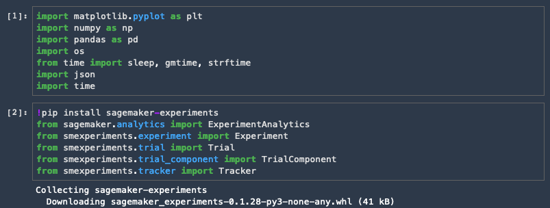
import matplotlib.pyplot as plt
import numpy as np
import pandas as pd
import os
from time import sleep, gmtime, strftime
import json
import time
!pip install sagemaker-experiments
from sagemaker.analytics import ExperimentAnalytics
from smexperiments.experiment import Experiment
from smexperiments.trial import Trial
from smexperiments.trial_component import TrialComponent
from smexperiments.tracker import Tracker
rawbucket= sess.default_bucket() # Alternatively you can use our custom bucket here.

prefix = 'sagemaker-modelmonitor' # use this prefix to store all files pertaining to this workshop.

dataprefix = prefix + '/data'
traindataprefix = prefix + '/train_data'
testdataprefix = prefix + '/test_data'
testdatanolabelprefix = prefix + '/test_data_no_label'
trainheaderprefix = prefix + '/train_headers'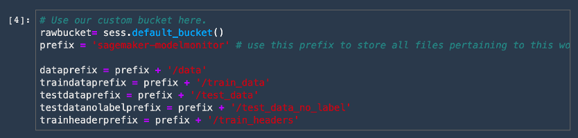
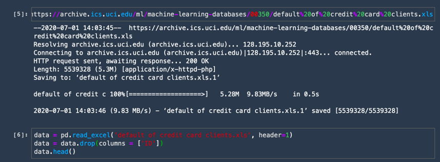
e. Download the dataset and import it using the pandas library. Copy and paste the following code into a new code cell and choose Run.
! wget https://archive.ics.uci.edu/ml/machine-learning-databases/00350/default%20of%20credit%20card%20clients.xls
data = pd.read_excel('default of credit card clients.xls', header=1)
data = data.drop(columns = ['ID'])
data.head()
f. Rename the last column as Label and extract the label column separately. For the Amazon SageMaker built-in XGBoost algorithm, the label column must be the first column in the dataframe. To make that change, copy and paste the following code into a new code cell and choose Run.
data.rename(columns={"default payment next month": "Label"}, inplace=True)
lbl = data.Label
data = pd.concat([lbl, data.drop(columns=['Label'])], axis = 1)
data.head()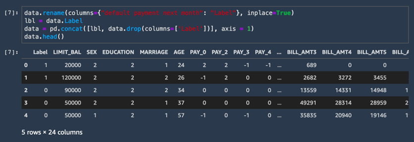
g. Upload the CSV dataset into an Amazon S3 bucket. Copy and paste the following code into a new code cell and choose Run.
if not os.path.exists('rawdata/rawdata.csv'):
    !mkdir rawdata
    data.to_csv('rawdata/rawdata.csv', index=None)
else:
    pass
# Upload the raw dataset
raw_data_location = sess.upload_data('rawdata', bucket=rawbucket, key_prefix=dataprefix)
print(raw_data_location)You're done! The code output displays the S3 bucket URI like the following example:
s3://sagemaker-us-east-2-ACCOUNT_NUMBER/sagemaker-modelmonitor/data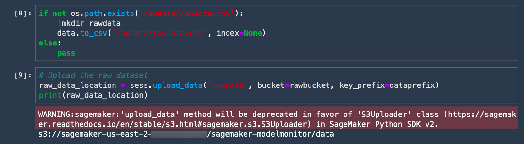
Step 4: Process the data using Amazon SageMaker Processing
In this step, you use Amazon SageMaker Processing to pre-process the dataset, including scaling the columns and splitting the dataset into train and test data. Amazon SageMaker Processing lets you run your preprocessing, postprocessing, and model evaluation workloads on fully managed infrastructure.
Complete the following steps to processs the data and generate features using Amazon SageMaker Processing.
Note: Amazon SageMaker Processing runs on separate compute instances from your notebook. This means you can continue to experiment and run code in your notebook while the processing job is under way. This will incur additional charges for the cost of the instance which is up and running for the duration of the processing job. The instances are automatically terminated by SageMaker once the processing job completes. For pricing details, see Amazon SageMaker Pricing.
Note: For more information, see Process Data and Evaluate Models in the Amazon SageMaker documentation.
a. Import the scikit-learn processing container. Copy and paste the following code into a new code cell and choose Run.
Note: Amazon SageMaker provides a managed container for scikit-learn. For more information, see Process Data and Evaluate Models with scikit-learn.
from sagemaker.sklearn.processing import SKLearnProcessor
sklearn_processor = SKLearnProcessor(framework_version='0.20.0',
                                     role=role,
                                     instance_type='ml.c4.xlarge',
                                     instance_count=1)
b. Copy and paste the following pre-processing script into a new cell and choose Run.
%%writefile preprocessing.py

import argparse
import os
import warnings

import pandas as pd
import numpy as np
from sklearn.model_selection import train_test_split
from sklearn.preprocessing import StandardScaler, MinMaxScaler
from sklearn.exceptions import DataConversionWarning
from sklearn.compose import make_column_transformer

warnings.filterwarnings(action='ignore', category=DataConversionWarning)

if __name__=='__main__':
    parser = argparse.ArgumentParser()
    parser.add_argument('--train-test-split-ratio', type=float, default=0.3)
    parser.add_argument('--random-split', type=int, default=0)
    args, _ = parser.parse_known_args()

    print('Received arguments {}'.format(args))

    input_data_path = os.path.join('/opt/ml/processing/input', 'rawdata.csv')

    print('Reading input data from {}'.format(input_data_path))
    df = pd.read_csv(input_data_path)
    df.sample(frac=1)

    COLS = df.columns
    newcolorder = ['PAY_AMT1','BILL_AMT1'] + list(COLS[1:])[:11] + list(COLS[1:])[12:17] + list(COLS[1:])[18:]

    split_ratio = args.train_test_split_ratio
    random_state=args.random_split

    X_train, X_test, y_train, y_test = train_test_split(df.drop('Label', axis=1), df['Label'],
                                                        test_size=split_ratio, random_state=random_state)

    preprocess = make_column_transformer(
        (['PAY_AMT1'], StandardScaler()),
        (['BILL_AMT1'], MinMaxScaler()),
    remainder='passthrough')

    print('Running preprocessing and feature engineering transformations')
    train_features = pd.DataFrame(preprocess.fit_transform(X_train), columns = newcolorder)
    test_features = pd.DataFrame(preprocess.transform(X_test), columns = newcolorder)

    # concat to ensure Label column is the first column in dataframe
    train_full = pd.concat([pd.DataFrame(y_train.values, columns=['Label']), train_features], axis=1)
    test_full = pd.concat([pd.DataFrame(y_test.values, columns=['Label']), test_features], axis=1)

    print('Train data shape after preprocessing: {}'.format(train_features.shape))
    print('Test data shape after preprocessing: {}'.format(test_features.shape))

    train_features_headers_output_path = os.path.join('/opt/ml/processing/train_headers', 'train_data_with_headers.csv')

    train_features_output_path = os.path.join('/opt/ml/processing/train', 'train_data.csv')

    test_features_output_path = os.path.join('/opt/ml/processing/test', 'test_data.csv')

    print('Saving training features to {}'.format(train_features_output_path))
    train_full.to_csv(train_features_output_path, header=False, index=False)
    print("Complete")

    print("Save training data with headers to {}".format(train_features_headers_output_path))
    train_full.to_csv(train_features_headers_output_path, index=False)

    print('Saving test features to {}'.format(test_features_output_path))
    test_full.to_csv(test_features_output_path, header=False, index=False)
print("Complete")c. Copy the preprocessing code over to the Amazon S3 bucket using the following code, then choose Run.
# Copy the preprocessing code over to the s3 bucket
codeprefix = prefix + '/code'
codeupload = sess.upload_data('preprocessing.py', bucket=rawbucket, key_prefix=codeprefix)
print(codeupload)

d. Specify where you want to store your training and test data after the SageMaker Processing job completes. Amazon SageMaker Processing automatically stores the data in the specified location.
train_data_location = rawbucket + '/' + traindataprefix
test_data_location = rawbucket+'/'+testdataprefix
print("Training data location = {}".format(train_data_location))
print("Test data location = {}".format(test_data_location))
e. Copy and paste the following code to start the Processing job. This code starts the job by calling sklearn_processor.run and extracts some optional metadata about the processing job, such as where the training and test outputs were stored.
from sagemaker.processing import ProcessingInput, ProcessingOutput

sklearn_processor.run(code=codeupload,
                      inputs=[ProcessingInput(
                        source=raw_data_location,
                        destination='/opt/ml/processing/input')],
                      outputs=[ProcessingOutput(output_name='train_data',
                                                source='/opt/ml/processing/train',
                               destination='s3://' + train_data_location),
                               ProcessingOutput(output_name='test_data',
                                                source='/opt/ml/processing/test',
                                               destination="s3://"+test_data_location),
                               ProcessingOutput(output_name='train_data_headers',
                                                source='/opt/ml/processing/train_headers',
                                               destination="s3://" + rawbucket + '/' + prefix + '/train_headers')],
                      arguments=['--train-test-split-ratio', '0.2']
                     )

preprocessing_job_description = sklearn_processor.jobs[-1].describe()

output_config = preprocessing_job_description['ProcessingOutputConfig']
for output in output_config['Outputs']:
    if output['OutputName'] == 'train_data':
        preprocessed_training_data = output['S3Output']['S3Uri']
    if output['OutputName'] == 'test_data':
        preprocessed_test_data = output['S3Output']['S3Uri']
Note the locations of the code, train and test data in the outputs provided to the processor. Also, note the arguments provided to the processing scripts.

Step 5: Create an Amazon SageMaker Experiment
Now that you have downloaded and staged your dataset in Amazon S3, you can create an Amazon SageMaker Experiment. An experiment is a collection of processing and training jobs related to the same machine learning project. Amazon SageMaker Experiments automatically manages and tracks your training runs for you.
Complete the following steps to create a new experiment.
Note: For more information, see Experiments in the Amazon SageMaker documentation.
a. Copy and paste the following code to create an experiment named Build-train-deploy-.
# Create a SageMaker Experiment
cc_experiment = Experiment.create(
    experiment_name=f"Build-train-deploy-{int(time.time())}",
    description="Predict credit card default from payments data",
    sagemaker_boto_client=sm)
print(cc_experiment)
Every training job is logged as a trial. Each trial is an iteration of your end-to-end training job. In addition to the training job, it can also track pre-processing and post-processing jobs as well as datasets and other metadata. A single experiment can include multiple trials which makes it easy for you to track multiple iterations over time within the Amazon SageMaker Studio Experiments pane.
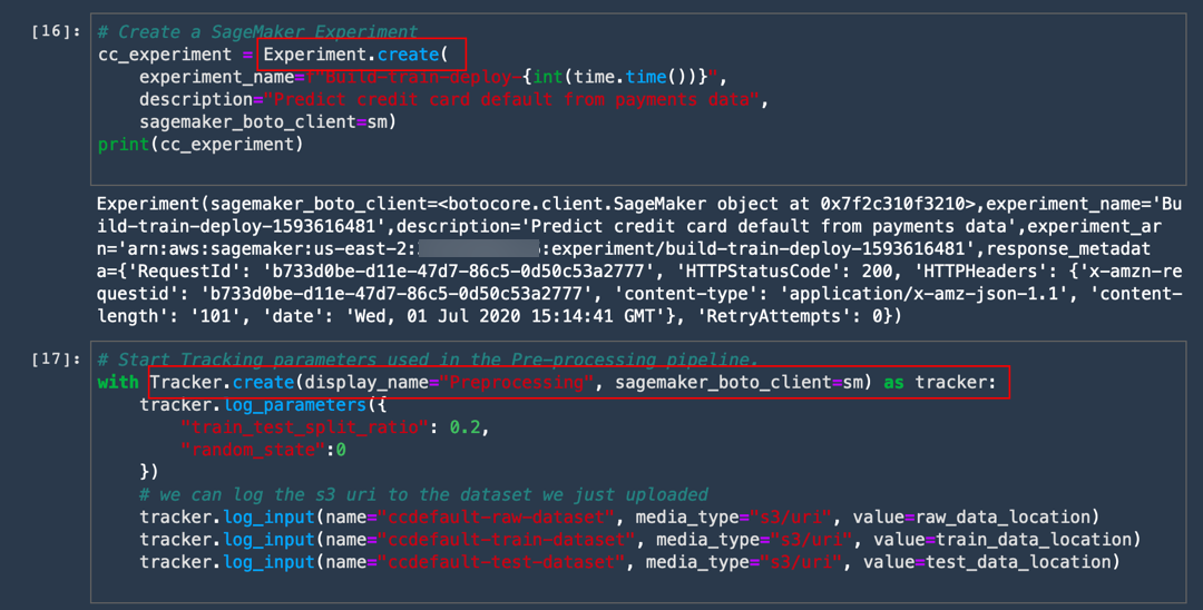
b. Copy and paste the following code to track your pre-processing job under Experiments as well as a step in the training pipeline.
# Start Tracking parameters used in the Pre-processing pipeline.
with Tracker.create(display_name="Preprocessing", sagemaker_boto_client=sm) as tracker:
    tracker.log_parameters({
        "train_test_split_ratio": 0.2,
        "random_state":0
    })
    # we can log the s3 uri to the dataset we just uploaded
    tracker.log_input(name="ccdefault-raw-dataset", media_type="s3/uri", value=raw_data_location)
    tracker.log_input(name="ccdefault-train-dataset", media_type="s3/uri", value=train_data_location)
    tracker.log_input(name="ccdefault-test-dataset", media_type="s3/uri", value=test_data_location)
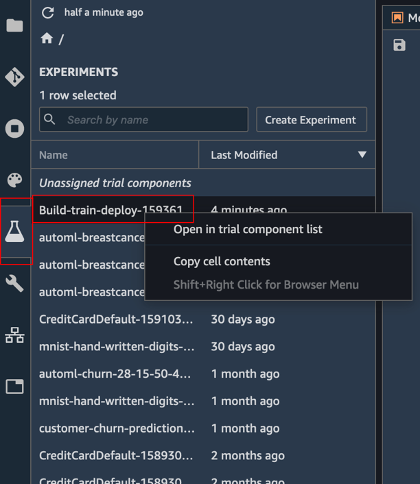
c. View the details of the experiment: In the Experiments pane, right-click the experiment named Build-train-deploy- and choose Open in trial components list.
d. Copy and paste the following code and choose Run. Then, take a closer look at the code:
To train an XGBoost classifier, you first import the XGBoost container maintained by Amazon SageMaker. Then, you log the training run under a Trial so SageMaker Experiments can track it under a Trial name. The pre-processing job is included under the same trial name since it is part of the pipeline. Next, create a SageMaker Estimator object, which automatically provisions the underlying instance type of your choosing, copies over the training data from the specified output location from the processing job, trains the model, and outputs the model artifacts.
from sagemaker.amazon.amazon_estimator import get_image_uri
container = get_image_uri(boto3.Session().region_name, 'xgboost', '1.0-1')
s3_input_train = sagemaker.s3_input(s3_data='s3://' + train_data_location, content_type='csv')
preprocessing_trial_component = tracker.trial_component

trial_name = f"cc-default-training-job-{int(time.time())}"
cc_trial = Trial.create(
        trial_name=trial_name,
            experiment_name=cc_experiment.experiment_name,
        sagemaker_boto_client=sm
    )

cc_trial.add_trial_component(preprocessing_trial_component)
cc_training_job_name = "cc-training-job-{}".format(int(time.time()))

xgb = sagemaker.estimator.Estimator(container,
                                    role,
                                    train_instance_count=1,
                                    train_instance_type='ml.m4.xlarge',
                                    train_max_run=86400,
                                    output_path='s3://{}/{}/models'.format(rawbucket, prefix),
                                    sagemaker_session=sess) # set to true for distributed training

xgb.set_hyperparameters(max_depth=5,
                        eta=0.2,
                        gamma=4,
                        min_child_weight=6,
                        subsample=0.8,
                        verbosity=0,
                        objective='binary:logistic',
                        num_round=100)

xgb.fit(inputs = {'train':s3_input_train},
       job_name=cc_training_job_name,
        experiment_config={
            "TrialName": cc_trial.trial_name, #log training job in Trials for lineage
            "TrialComponentDisplayName": "Training",
        },
        wait=True,
    )
time.sleep(2)
The training job will take about 70 seconds to complete. You should see the following output.
Completed - Training job completed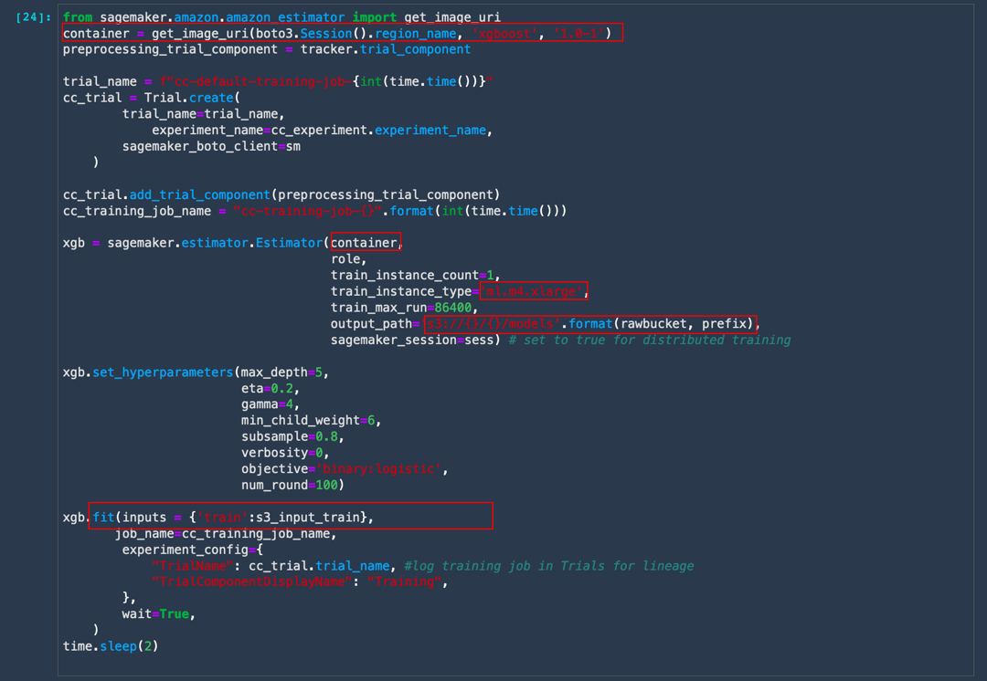
e. In the left toolbar, choose Experiment. Right-click the Build-train-deploy- experiment and choose Open in trial components list. Amazon SageMaker Experiments captures all the runs including any failed training runs.
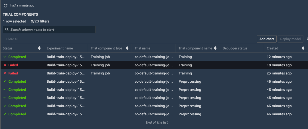
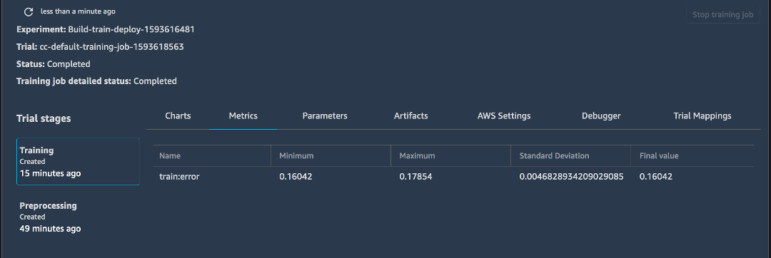
f. Right-click one of the completed Training jobs and choose Open in Trial Details to explore the associated metadata with the training job.
Note: You may need to refresh the page to see the latest results.
Step 6: Deploy the model for offline inference
In your preprocessing step, you generated some test data. In this step, you generate offline or batch inference from the trained model to evaluate the model performance on unseen test data.
Complete the following steps to deploy the model for offline inference.
Note: For more information, see Batch Transform in the Amazon SageMaker documentation.
a. Copy and paste the following code and choose Run.
This step copies the test dataset over from the Amazon S3 location into your local folder.
test_data_path = 's3://' + test_data_location + '/test_data.csv'
! aws s3 cp $test_data_path .
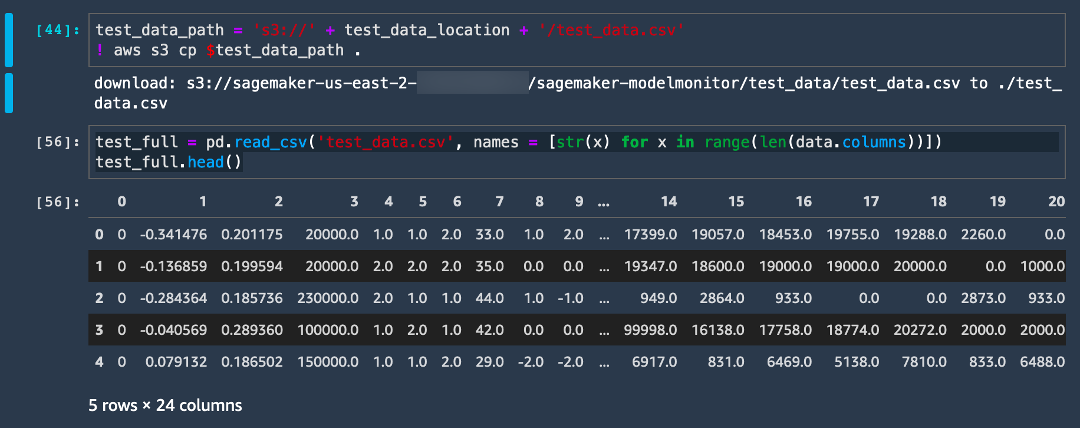
b. Copy and paste the following code and choose Run.
test_full = pd.read_csv('test_data.csv', names = [str(x) for x in range(len(data.columns))])
test_full.head()
c. Copy and paste the following code and choose Run. This step extracts the label column.
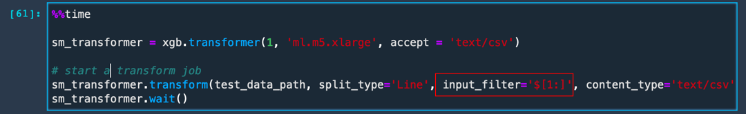
label = test_full['0'] d. Copy and paste the following code and choose Run to create the Batch Transform job. Then, take a closer look at the code:
Like the training job, SageMaker provisions all the underlying resources, copies over the trained model artifacts, sets up a Batch endpoint locally, copies over the data, and runs inferences on the data and pushes the outputs to Amazon S3. Note that by setting the input_filter, you are letting Batch Transform know to neglect the first column in the test data which is the label column.
%%time

sm_transformer = xgb.transformer(1, 'ml.m5.xlarge', accept = 'text/csv')

# start a transform job
sm_transformer.transform(test_data_path, split_type='Line', input_filter='$[1:]', content_type='text/csv')
sm_transformer.wait()
The Batch Transform job will take about 4 minutes to complete after which you can evaluate the model results.
e. Copy and run the following code to evaluate the model metrics. Then, take a closer look at the code:
First, you define a function that pulls the output of the Batch Transform job, which is contained in a file with a .out extension from the Amazon S3 bucket. Then, you extract the predicted labels into a dataframe and append the true labels to this dataframe.
import json
import io
from urllib.parse import urlparse
def get_csv_output_from_s3(s3uri, file_name):
parsed_url = urlparse(s3uri)
bucket_name = parsed_url.netloc
prefix = parsed_url.path[1:]
s3 = boto3.resource('s3')
obj = s3.Object(bucket_name, '{}/{}'.format(prefix, file_name))
return obj.get()["Body"].read().decode('utf-8')
output = get_csv_output_from_s3(sm_transformer.output_path, 'test_data.csv.out')
output_df = pd.read_csv(io.StringIO(output), sep=",", header=None)
output_df.head(8)
output_df['Predicted']=np.round(output_df.values)
output_df['Label'] = label
from sklearn.metrics import confusion_matrix, accuracy_score
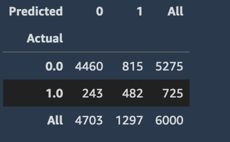
confusion_matrix = pd.crosstab(output_df['Predicted'], output_df['Label'], rownames=['Actual'], colnames=['Predicted'], margins = True)
confusion_matrix
You should see an output similar to the image, which shows the total number of Predicted True and False values compared to the Actual values.
f. Use the following code to extract both the baseline model accuracy and the model accuracy.
Note: A helpful model for the baseline accuracy can be the fraction of non-default cases. A model that always predicts that a user will not default has that accuracy.
print("Baseline Accuracy = {}".format(1- np.unique(data['Label'], return_counts=True)[1][1]/(len(data['Label']))))
print("Accuracy Score = {}".format(accuracy_score(label, output_df['Predicted'])))
The results show that a simple model can already beat the baseline accuracy. In order to improve the results, you can tune the hyperparameters. You can use hyperparameter optimization (HPO) on SageMaker for automatic model tuning. To learn more, see How Hyperparameter Tuning Works.
Note: Although it is not included in this tutorial, you also have the option of including Batch Transform as part of your trial. When you call the .transform function, simply pass in the experiment_config as you did for the Training job. Amazon SageMaker automatically associates the Batch Transform as a trial component.

Step 7: Deploy the model as an endpoint and set up data capture
In this step, you deploy the model as a RESTful HTTPS endpoint to serve live inferences. Amazon SageMaker automatically handles the model hosting and creation of the endpoint for you.
Complete the following steps to deploy the model as an endpoint and set up data capture.
Note: For more information, see Deploy Models for Inference in the Amazon SageMaker documentation.
a. Copy and paste the following code and choose Run.
from sagemaker.model_monitor import DataCaptureConfig
from sagemaker import RealTimePredictor
from sagemaker.predictor import csv_serializer

sm_client = boto3.client('sagemaker')

latest_training_job = sm_client.list_training_jobs(MaxResults=1,
                                                SortBy='CreationTime',
                                                SortOrder='Descending')

training_job_name=TrainingJobName=latest_training_job['TrainingJobSummaries'][0]['TrainingJobName']

training_job_description = sm_client.describe_training_job(TrainingJobName=training_job_name)

model_data = training_job_description['ModelArtifacts']['S3ModelArtifacts']
container_uri = training_job_description['AlgorithmSpecification']['TrainingImage']

# create a model.
def create_model(role, model_name, container_uri, model_data):
    return sm_client.create_model(
        ModelName=model_name,
        PrimaryContainer={
        'Image': container_uri,
        'ModelDataUrl': model_data,
        },
        ExecutionRoleArn=role)


try:
    model = create_model(role, training_job_name, container_uri, model_data)
except Exception as e:
        sm_client.delete_model(ModelName=training_job_name)
        model = create_model(role, training_job_name, container_uri, model_data)


print('Model created: '+model['ModelArn'])

b. To specify the data configuration settings, copy and paste the following code and choose Run.
This code tells SageMaker to capture 100% of the inference payloads received by the endpoint, capture both inputs and outputs, and also note the input content type as csv.
s3_capture_upload_path = 's3://{}/{}/monitoring/datacapture'.format(rawbucket, prefix)
data_capture_configuration = {
    "EnableCapture": True,
    "InitialSamplingPercentage": 100,
    "DestinationS3Uri": s3_capture_upload_path,
    "CaptureOptions": [
        { "CaptureMode": "Output" },
        { "CaptureMode": "Input" }
    ],
    "CaptureContentTypeHeader": {
       "CsvContentTypes": ["text/csv"],
       "JsonContentTypes": ["application/json"]}}
c. Copy and paste the following code and choose Run. This step creates an endpoint configuration and deploys the endpoint. In the code, you can specify instance type and whether you want to send all the traffic to this endpoint, etc.
def create_endpoint_config(model_config, data_capture_config):
    return sm_client.create_endpoint_config(
                                                EndpointConfigName=model_config,
                                                ProductionVariants=[
                                                        {
                                                            'VariantName': 'AllTraffic',
                                                            'ModelName': model_config,
                                                            'InitialInstanceCount': 1,
                                                            'InstanceType': 'ml.m4.xlarge',
                                                            'InitialVariantWeight': 1.0,
                                                },

                                                    ],
                                                DataCaptureConfig=data_capture_config
                                                )


try:
    endpoint_config = create_endpoint_config(training_job_name, data_capture_configuration)
except Exception as e:
    sm_client.delete_endpoint_config(EndpointConfigName=endpoint)
    endpoint_config = create_endpoint_config(training_job_name, data_capture_configuration)

print('Endpoint configuration created: '+ endpoint_config['EndpointConfigArn'])
d. Copy and paste the following code and choose Run to create the endpoint.
# Enable data capture, sampling 100% of the data for now. Next we deploy the endpoint in the correct VPC.

endpoint_name = training_job_name
def create_endpoint(endpoint_name, config_name):
    return sm_client.create_endpoint(
                                    EndpointName=endpoint_name,
                                    EndpointConfigName=training_job_name
                                )


try:
    endpoint = create_endpoint(endpoint_name, endpoint_config)
except Exception as e:
    sm_client.delete_endpoint(EndpointName=endpoint_name)
    endpoint = create_endpoint(endpoint_name, endpoint_config)

print('Endpoint created: '+ endpoint['EndpointArn'])

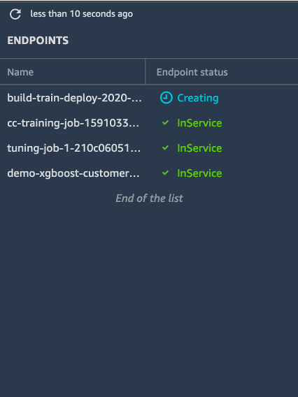
e. In the left toolbar, choose Endpoints. The Endpoints list displays all of the endpoints in service.
Notice the build-train-deploy endpoint shows a status of Creating. To deploy the model, Amazon SageMaker must first copy your model artifacts and inference image onto the instance and set up a HTTPS endpoint to inferface with client applications or RESTful APIs.
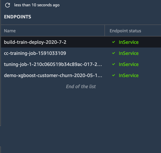
Once the endpoint is created, the status changes to InService. (Note that creating an endpoint may take about 5-10 minutes.)
Note: You may need to click Refresh to get the updated status.
f. In the JupyterLab Notebook, copy and run the following code to take a sample of the test dataset. This code takes the first 10 rows.
!head -10 test_data.csv > test_sample.csvg. Run the following code to send some inference requests to this endpoint.
Note: If you specified a different endpoint name, you will need to replace endpoint below with your endpoint name.
from sagemaker import RealTimePredictor
from sagemaker.predictor import csv_serializer

predictor = RealTimePredictor(endpoint=endpoint_name, content_type = 'text/csv')

with open('test_sample.csv', 'r') as f:
    for row in f:
        payload = row.rstrip('\n')
        response = predictor.predict(data=payload[2:])
        sleep(0.5)
print('done!')
h. Run the following code to verify that Model Monitor is correctly capturing the incoming data.
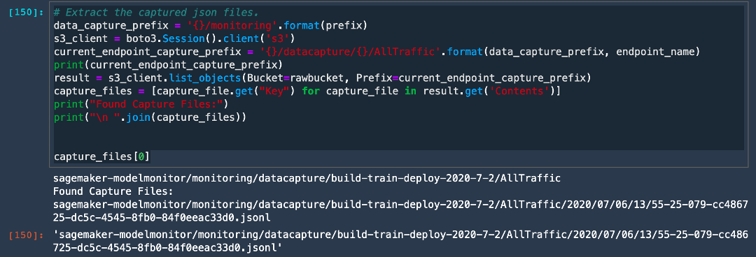
In the code, the current_endpoint_capture_prefix captures the directory path where your ModelMonitor outputs are stored. Navigate to your Amazon S3 bucket, to see if the prediction requests are being captured. Note that this location should match the s3_capture_upload_path in the code above.
# Extract the captured json files.
data_capture_prefix = '{}/monitoring'.format(prefix)
s3_client = boto3.Session().client('s3')
current_endpoint_capture_prefix = '{}/datacapture/{}/AllTraffic'.format(data_capture_prefix, endpoint_name)
print(current_endpoint_capture_prefix)
result = s3_client.list_objects(Bucket=rawbucket, Prefix=current_endpoint_capture_prefix)
capture_files = [capture_file.get("Key") for capture_file in result.get('Contents')]
print("Found Capture Files:")
print("\n ".join(capture_files))


capture_files[0]
The captured output indicates that data capture is configured and saving the incoming requests.
Note: If you initially see a Null response, the data may not have been synchronously loaded onto the Amazon S3 path when you first initialized the data capture. Wait about a minute and try again.
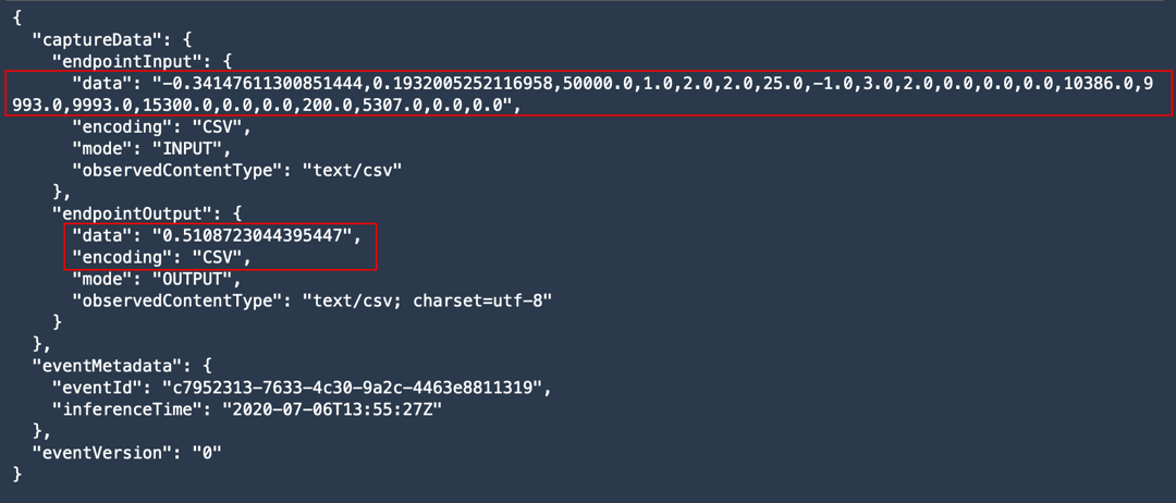
i. Run the following code to extract the content of one of the json files and view the captured outputs.
# View contents of the captured file.
def get_obj_body(bucket, obj_key):
    return s3_client.get_object(Bucket=rawbucket, Key=obj_key).get('Body').read().decode("utf-8")

capture_file = get_obj_body(rawbucket, capture_files[0])
print(json.dumps(json.loads(capture_file.split('\n')[5]), indent = 2, sort_keys =True))
The output indicates that data capture is capturing both the input payload and the output of the model.
Step 8: Monitor the endpoint with SageMaker Model Monitor
In this step, you enable SageMaker Model Monitor to monitor the deployed endpoint for data drift. To do so, you compare the payload and outputs sent to the model against a baseline and determine whether there is any drift in the input data, or the label.
Complete the following steps to enable model monitoring.
Note: For more information, see Amazon SageMaker Model Monitor in the Amazon SageMaker documentation.
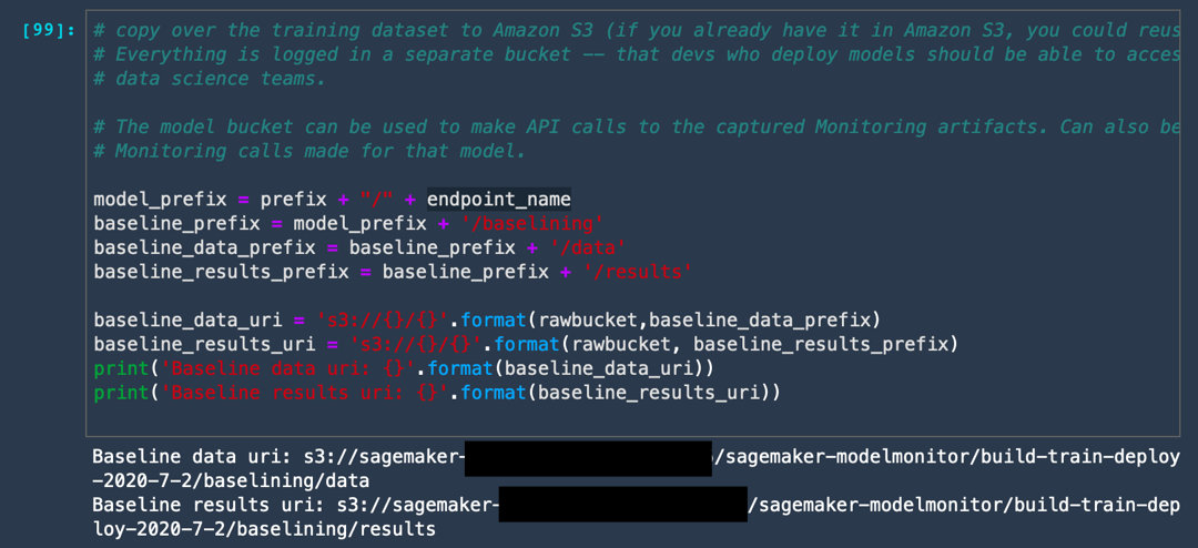
a. Run the following code to create a folder in your Amazon S3 bucket to store the outputs of the Model Monitor.
This code creates two folders: one folder stores the baseline data which you used for training your model; the second folder stores any violations from that baseline.
model_prefix = prefix + "/" + endpoint_name
baseline_prefix = model_prefix + '/baselining'
baseline_data_prefix = baseline_prefix + '/data'
baseline_results_prefix = baseline_prefix + '/results'

baseline_data_uri = 's3://{}/{}'.format(rawbucket,baseline_data_prefix)
baseline_results_uri = 's3://{}/{}'.format(rawbucket, baseline_results_prefix)
train_data_header_location = "s3://" + rawbucket + '/' + prefix + '/train_headers'
print('Baseline data uri: {}'.format(baseline_data_uri))
print('Baseline results uri: {}'.format(baseline_results_uri))
print(train_data_header_location)
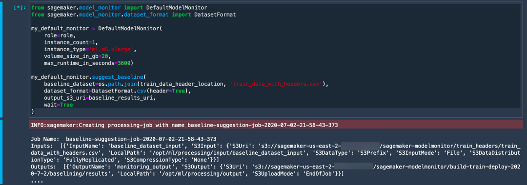
b. Run the following code to set up a baseline job for Model Monitor to capture the statistics of the training data. To do this, Model Monitor uses the deequ library built on top of Apache Spark for conducting unit tests on data.
from sagemaker.model_monitor import DefaultModelMonitor
from sagemaker.model_monitor.dataset_format import DatasetFormat

my_default_monitor = DefaultModelMonitor(
    role=role,
    instance_count=1,
    instance_type='ml.m5.xlarge',
    volume_size_in_gb=20,
    max_runtime_in_seconds=3600)

my_default_monitor.suggest_baseline(
    baseline_dataset=os.path.join(train_data_header_location, 'train_data_with_headers.csv'),
    dataset_format=DatasetFormat.csv(header=True),
    output_s3_uri=baseline_results_uri,
    wait=True
)
Model Monitor sets up a separate instance, copies over the training data, and generates some statistics. The service generates a lot of Apache Spark logs, which you can ignore. Once the job is completed, you will see a Spark job completed output.
c. Run the following code to look at the outputs generated by the baseline job.
s3_client = boto3.Session().client('s3')
result = s3_client.list_objects(Bucket=rawbucket, Prefix=baseline_results_prefix)
report_files = [report_file.get("Key") for report_file in result.get('Contents')]
print("Found Files:")
print("\n ".join(report_files))
baseline_job = my_default_monitor.latest_baselining_job
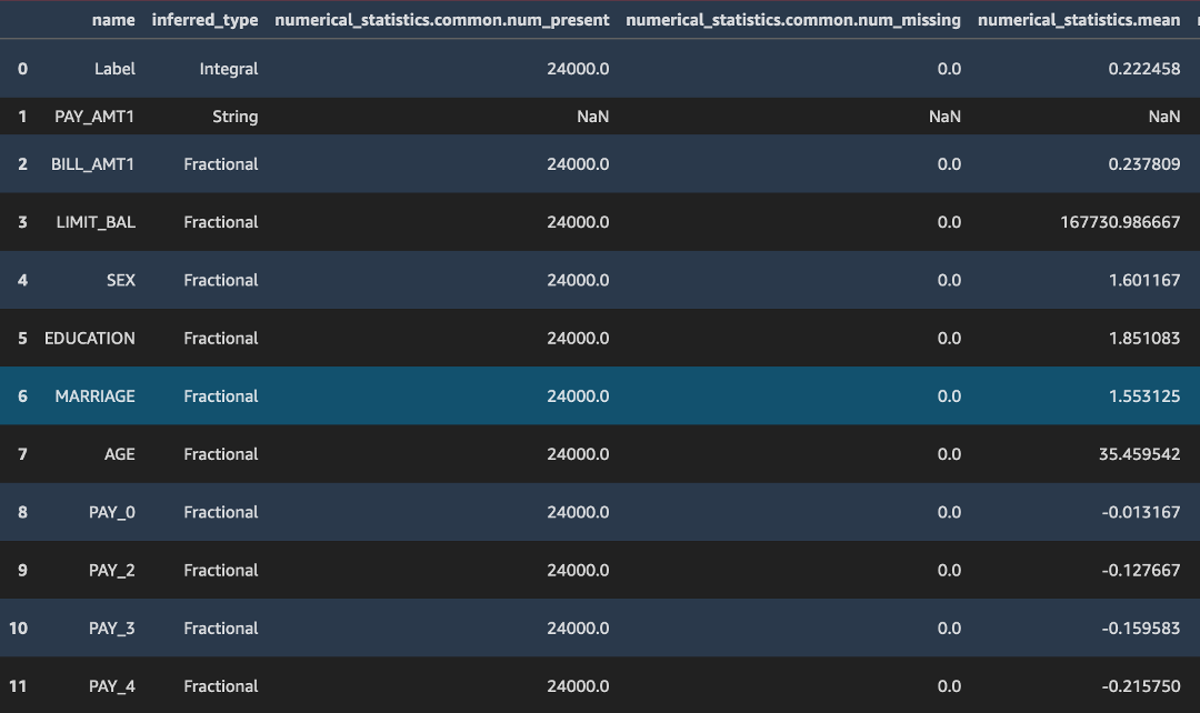
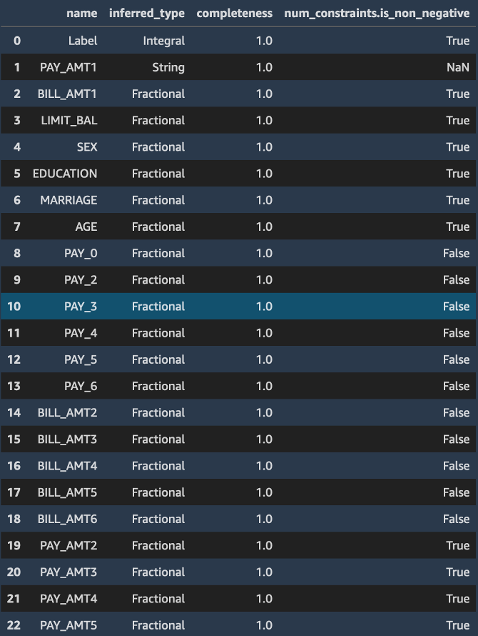
schema_df = pd.io.json.json_normalize(baseline_job.baseline_statistics().body_dict["features"])
schema_df
You will see two files: constraints.json and statistics.json. Next, dive deeper into their contents.

The code above converts the json output in /statistics.json into a pandas dataframe. Note how the deequ library infers the data type of the column, the presence or absence of Null or missing values, and statistical parameters such as the mean, min, max, sum, standard deviation, and sketch parameters for an input data stream.
Likewise, the constraints.json file consists of a number of constraints the training dataset obeys such as non-negativity of values, and the data type of the feature field.
constraints_df = pd.io.json.json_normalize(baseline_job.suggested_constraints().body_dict["features"])
constraints_df
d. Run the following code to set up the frequency for endpoint monitoring.
You can specify daily or hourly. This code specifies an hourly frequency, but you may want to change this for production applications as hourly frequency will generate a lot of data. Model Monitor will produce a report consisting of all the violations it finds.
reports_prefix = '{}/reports'.format(prefix)
s3_report_path = 's3://{}/{}'.format(rawbucket,reports_prefix)
print(s3_report_path)

from sagemaker.model_monitor import CronExpressionGenerator
from time import gmtime, strftime

mon_schedule_name = 'Built-train-deploy-model-monitor-schedule-' + strftime("%Y-%m-%d-%H-%M-%S", gmtime())
my_default_monitor.create_monitoring_schedule(
    monitor_schedule_name=mon_schedule_name,
    endpoint_input=predictor.endpoint,
    output_s3_uri=s3_report_path,
    statistics=my_default_monitor.baseline_statistics(),
    constraints=my_default_monitor.suggested_constraints(),
    schedule_cron_expression=CronExpressionGenerator.hourly(),
    enable_cloudwatch_metrics=True,

)
Note that this code enables Amazon CloudWatch Metrics, which instructs Model Monitor to send outputs to CloudWatch. You can use this approach to trigger alarms using CloudWatch Alarms to let engineers or admins know when data drift has been detected.

Step 9: Test SageMaker Model Monitor performance
In this step, you evaluate Model Monitor against some sample data. Instead of sending the test payload as is, you modify the distribution of several features in the test payload to test that Model Monitor can detect the change.
Complete the following steps to test the Model Monitor performance.
Note: For more information, see Amazon SageMaker Model Monitor in the Amazon SageMaker documentation.
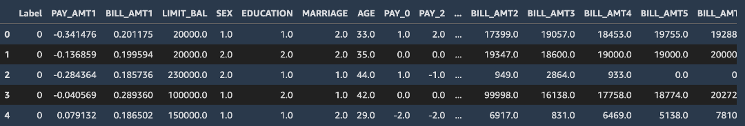
a. Run the following code to import the test data and generate some modified sample data.
COLS = data.columns
test_full = pd.read_csv('test_data.csv', names = ['Label'] +['PAY_AMT1','BILL_AMT1'] + list(COLS[1:])[:11] + list(COLS[1:])[12:17] + list(COLS[1:])[18:]
)
test_full.head()
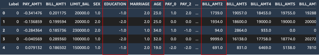
b. Run the following code to change a few columns. Note the differences marked in red in the image here from the previous step. Drop the label column and save the modified sample test data.
faketestdata = test_full
faketestdata['EDUCATION'] = -faketestdata['EDUCATION'].astype(float)
faketestdata['BILL_AMT2']= (faketestdata['BILL_AMT2']//10).astype(float)
faketestdata['AGE']= (faketestdata['AGE']-10).astype(float)

faketestdata.head()
faketestdata.drop(columns=['Label']).to_csv('test-data-input-cols.csv', index = None, header=None)
c. Run the following code to repeatedly invoke the endpoint with this modified dataset.
from threading import Thread

runtime_client = boto3.client('runtime.sagemaker')

# (just repeating code from above for convenience/ able to run this section independently)
def invoke_endpoint(ep_name, file_name, runtime_client):
    with open(file_name, 'r') as f:
        for row in f:
            payload = row.rstrip('\n')
            response = runtime_client.invoke_endpoint(EndpointName=ep_name,
                                          ContentType='text/csv',
                                          Body=payload)
            time.sleep(1)

def invoke_endpoint_forever():
    while True:
        invoke_endpoint(endpoint, 'test-data-input-cols.csv', runtime_client)

thread = Thread(target = invoke_endpoint_forever)
thread.start()
# Note that you need to stop the kernel to stop the invocations
d. Run the following code to check the status of the Model Monitor job.
desc_schedule_result = my_default_monitor.describe_schedule()
print('Schedule status: {}'.format(desc_schedule_result['MonitoringScheduleStatus']))
You should see an output of Schedule status: Scheduled
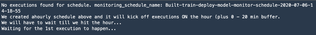
e. Run the following code to check every 10 minutes if any monitoring outputs have been generated. Note that the first job may run with a buffer of about 20 minutes.
mon_executions = my_default_monitor.list_executions()
print("We created ahourly schedule above and it will kick off executions ON the hour (plus 0 - 20 min buffer.\nWe will have to wait till we hit the hour...")

while len(mon_executions) == 0:
    print("Waiting for the 1st execution to happen...")
    time.sleep(600)
    mon_executions = my_default_monitor.list_executions()
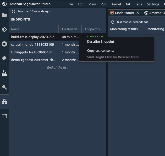
f. In the left toolbar of Amazon SageMaker Studio, choose Endpoints. Right-click the build-train-deploy endpoint and choose Describe Endpoint.
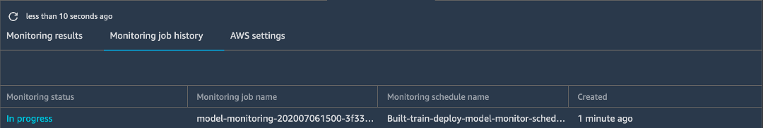
g. Choose Monitoring job history. Notice that the Monitoring status shows In progress.
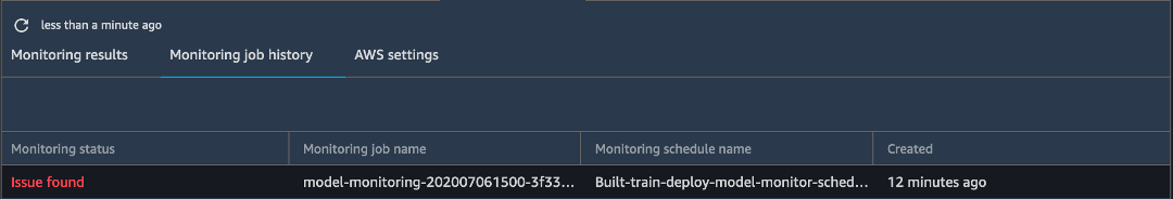
Once the job is complete, the Monitoring status displays Issue found (for any issues found).
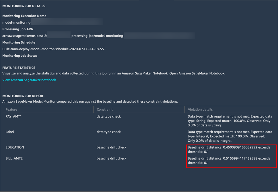
h. Double-click the issue to view details. You can see that Model Monitor detected large baseline drifts in the EDUCATION and BILL_AMT2 fields that you previously modified.
Model Monitor also detected some differences in data types in two other fields. The training data consists of integer labels, but the XGBoost model predicts a probability score. Therefore, Model Monitor reported a mismatch.
i. In your JupyterLab Notebook, run the following cells to see the output from Model Monitor.
latest_execution = mon_executions[-1] # latest execution's index is -1, second to last is -2 and so on..
time.sleep(60)
latest_execution.wait(logs=False)

print("Latest execution status: {}".format(latest_execution.describe()['ProcessingJobStatus']))
print("Latest execution result: {}".format(latest_execution.describe()['ExitMessage']))

latest_job = latest_execution.describe()
if (latest_job['ProcessingJobStatus'] != 'Completed'):
        print("====STOP==== \n No completed executions to inspect further. Please wait till an execution completes or investigate previously reported failures.")

j. Run the following code to view the reports generated by Model Monitor.
report_uri=latest_execution.output.destination
print('Report Uri: {}'.format(report_uri))
from urllib.parse import urlparse
s3uri = urlparse(report_uri)
report_bucket = s3uri.netloc
report_key = s3uri.path.lstrip('/')
print('Report bucket: {}'.format(report_bucket))
print('Report key: {}'.format(report_key))
s3_client = boto3.Session().client('s3')
result = s3_client.list_objects(Bucket=rawbucket, Prefix=report_key)
report_files = [report_file.get("Key") for report_file in result.get('Contents')]
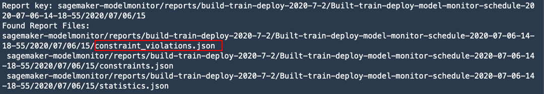
print("Found Report Files:")
print("\n ".join(report_files))
You can see that in addition to statistics.json and constraints.json, there is a new file generated named constraint_violations.json. The contents of this file were displayed above in Amazon SageMaker Studio (Step g).
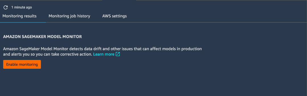
Note: Once you set up data capture, Amazon SageMaker Studio automatically creates a notebook for you that contains the code above to run monitoring jobs. To access the notebook, right-click the endpoint and choose Describe Endpoint. On the Monitoring results tab, choose Enable Monitoring. This step automatically opens a Jupyter notebook containing the code you authored above.
Step 10. Clean up
In this step, you terminate the resources you used in this lab.
Important: Terminating resources that are not actively being used reduces costs and is a best practice. Not terminating your resources will result in charges to your account.
a. Delete monitoring schedules: In your Jupyter notebook, copy and paste the following code and choose Run.
Note: You cannot delete the Model Monitor endpoint until all of the monitoring jobs associated with the endpoint are deleted.
my_default_monitor.delete_monitoring_schedule()
time.sleep(10) # actually wait for the deletion
b. Delete your endpoint: In your Jupyter notebook, copy and paste the following code and choose Run.
Note: Make sure you have first deleted all monitoring jobs associated with the endpoint.
sm.delete_endpoint(EndpointName = endpoint_name)If you want to clean up all training artifacts (models, preprocessed data sets, etc.), copy and paste the following code into your code cell and choose Run.
Note: Make sure to replace ACCOUNT_NUMBER with your account number.
%%sh
aws s3 rm --recursive s3://sagemaker-us-east-2-ACCOUNT_NUMBER/sagemaker-modelmonitor/data
Conclusion
You can continue your machine learning journey with SageMaker by following the next steps section below.