Build a semantic content recommendation system with Amazon SageMaker

Download and prepare the dataset

Train and deploy the topic model

Train and deploy the content recommendation model

In this module, you use the built-in Amazon SageMaker k-Nearest Neighbors (k-NN) Algorithm to train the content recommendation model.

Amazon SageMaker K-Nearest Neighbors (k-NN) is a non-parametric, index-based, supervised learning algorithm that can be used for classification and regression tasks. For classification, the algorithm queries the k closest points to the target and returns the most frequently used label of their class as the predicted label. For regression problems, the algorithm returns the average of the predicted values returned by the k closest neighbors.

Training with the k-NN algorithm has three steps: sampling, dimension reduction, and index building. Sampling reduces the size of the initial dataset so that it fits into memory. For dimension reduction, the algorithm decreases the feature dimension of the data to reduce the footprint of the k-NN model in memory and inference latency. We provide two methods of dimension reduction methods: random projection and the fast Johnson-Lindenstrauss transform. Typically, you use dimension reduction for high-dimensional (d >1000) datasets to avoid the “curse of dimensionality” that troubles the statistical analysis of data that becomes sparse as dimensionality increases. The main objective of k-NN's training is to construct the index. The index enables efficient lookups of distances between points whose values or class labels have not yet been determined and the k nearest points to use for inference.

In the following steps, you specify your k-NN algorithm for the training job, set the hyperparameter values to tune the model, and run the model. Then, you deploy the model to an endpoint managed by Amazon SageMaker to make predictions.

Time to Complete Module: 20 Minutes

Step 1. Create and run the training job

In the previous module, you created topic vectors. In this module, you build and deploy the content recommendation module which retains an index of the topic vectors.

First, create a dictionary which links the shuffled labels to the original labels in the training data. In your notebook, copy and paste the following code and choose Run.

labels = newidx 
labeldict = dict(zip(newidx,idx))

Next, store the training data in your S3 bucket using the following code:

import io
import sagemaker.amazon.common as smac


print('train_features shape = ', predictions.shape)
print('train_labels shape = ', labels.shape)
buf = io.BytesIO()
smac.write_numpy_to_dense_tensor(buf, predictions, labels)
buf.seek(0)

bucket = BUCKET
prefix = PREFIX
key = 'knn/train'
fname = os.path.join(prefix, key)
print(fname)
boto3.resource('s3').Bucket(bucket).Object(fname).upload_fileobj(buf)
s3_train_data = 's3://{}/{}/{}'.format(bucket, prefix, key)
print('uploaded training data location: {}'.format(s3_train_data))

Next, use the following helper function to create a k-NN estimator much like the NTM estimator you created in Module 3.

def trained_estimator_from_hyperparams(s3_train_data, hyperparams, output_path, s3_test_data=None):
    """
    Create an Estimator from the given hyperparams, fit to training data, 
    and return a deployed predictor
    
    """
    # set up the estimator
    knn = sagemaker.estimator.Estimator(get_image_uri(boto3.Session().region_name, "knn"),
        get_execution_role(),
        train_instance_count=1,
        train_instance_type='ml.c4.xlarge',
        output_path=output_path,
        sagemaker_session=sagemaker.Session())
    knn.set_hyperparameters(**hyperparams)
    
    # train a model. fit_input contains the locations of the train and test data
    fit_input = {'train': s3_train_data}
    knn.fit(fit_input)
    return knn

hyperparams = {
    'feature_dim': predictions.shape[1],
    'k': NUM_NEIGHBORS,
    'sample_size': predictions.shape[0],
    'predictor_type': 'classifier' ,
    'index_metric':'COSINE'
}
output_path = 's3://' + bucket + '/' + prefix + '/knn/output'
knn_estimator = trained_estimator_from_hyperparams(s3_train_data, hyperparams, output_path)

While the training job runs, take a closer look at the parameters in the helper function.

The Amazon SageMaker k-NN algorithm offers a number of different distance metrics for calculating the nearest neighbors. One popular metric that is used in natural language processing is the cosine distance. Mathematically, the cosine “similarity” between two vectors A and B is given by the following equation:

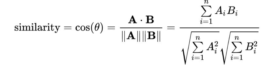
By setting the index_metric to COSINE, Amazon SageMaker automatically uses the cosine similarity for computing the nearest neighbors. The default distance is the L2 norm, which is the standard Euclidean distance. Note that, at publication, COSINE is only supported for faiss.IVFFlat index type and not the faiss.IVFPQ indexing method.

You should see the following output in your terminal.

Completed - Training job completed

Success! Since you want this model to return the nearest neighbors given a particular test topic, you need to deploy it as a live hosted endpoint.

Step 2. Deploy the content recommendation model

As you did with the NTM model, define the following helper function for the k-NN model to launch the endpoint. In the helper function, the accept token applications/jsonlines; verbose=true tells the k-NN model to return all the cosine distances instead of just the closest neighbor. To build a recommendation engine, you need to get the top-k suggestions by the model, for which youneed to set the verbose parameter to true, instead of the default, false.

Copy and paste the following code into your notebook and choose Run.

def predictor_from_estimator(knn_estimator, estimator_name, instance_type, endpoint_name=None): 
    knn_predictor = knn_estimator.deploy(initial_instance_count=1, instance_type=instance_type,
                                        endpoint_name=endpoint_name,
                                        accept="application/jsonlines; verbose=true")
    knn_predictor.content_type = 'text/csv'
    knn_predictor.serializer = csv_serializer
    knn_predictor.deserializer = json_deserializer
    return knn_predictor
import time

instance_type = 'ml.m4.xlarge'
model_name = 'knn_%s'% instance_type
endpoint_name = 'knn-ml-m4-xlarge-%s'% (str(time.time()).replace('.','-'))
print('setting up the endpoint..')
knn_predictor = predictor_from_estimator(knn_estimator, model_name, instance_type, endpoint_name=endpoint_name)

Next, preprocess the test data so that you can run inferences.

Copy and paste the following code into your notebook and choose Run.

def preprocess_input(text):
    text = strip_newsgroup_header(text)
    text = strip_newsgroup_quoting(text)
    text = strip_newsgroup_footer(text)
    return text    
    
test_data_prep = []
for i in range(len(newsgroups_test)):
    test_data_prep.append(preprocess_input(newsgroups_test[i]))
test_vectors = vectorizer.fit_transform(test_data_prep)

test_vectors = np.array(test_vectors.todense())
test_topics = []
for vec in test_vectors:
    test_result = ntm_predictor.predict(vec)
    test_topics.append(test_result['predictions'][0]['topic_weights'])

topic_predictions = []
for topic in test_topics:
    result = knn_predictor.predict(topic)
    cur_predictions = np.array([int(result['labels'][i]) for i in range(len(result['labels']))])
    topic_predictions.append(cur_predictions[::-1][:10])

In the last step of this module, you explore your content recommendation model.

Step 3. Explore content recommendation model
Step 3. Explore content recommendation model

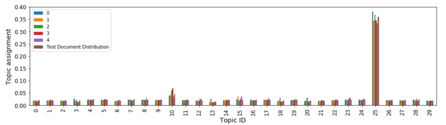
Now that you've obtained the predictions, you can plot the topic distributions of the test topics, compared to the closest k topics recommended by the k-NN model.

Copy and paste the following code into your notebook and choose Run.
```
# set your own k.
def plot_topic_distribution(topic_num, k = 5):
    
    closest_topics = [predictions[labeldict[x]] for x in topic_predictions[topic_num][:k]]
    closest_topics.append(np.array(test_topics[topic_num]))
    closest_topics = np.array(closest_topics)
    df = pd.DataFrame(closest_topics.T)
    df.rename(columns ={k:"Test Document Distribution"}, inplace=True)
    fs = 12
    df.plot(kind='bar', figsize=(16,4), fontsize=fs)
    plt.ylabel('Topic assignment', fontsize=fs+2)
    plt.xlabel('Topic ID', fontsize=fs+2)
    plt.show()
```
Run the following code to plot the topic distribution:
```
plot_topic_distribution(18)
```
Now, try some other topics. Run the following code cells:
```
plot_topic_distribution(25)
```
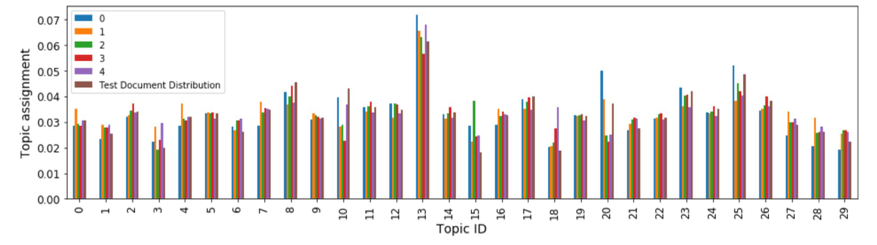
```
plot_topic_distribution(5000)
```
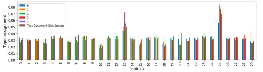
Your plots may look somewhat different based on the number of topics (NUM_TOPICS) you choose. But overall, these plots show that the topic distribution of the nearest neighbor documents found using Cosine similarity by the k-NN model is pretty similar to the topic distribution of the test document we fed into the model.

The results suggest that k-NN may be a good way to build a semantic based information retrieval system by first embedding the documents into topic vectors and then using a k-NN model to serve the recommendations.