In the news

ML Solutions Lab 'Coverage Classification' Q&A

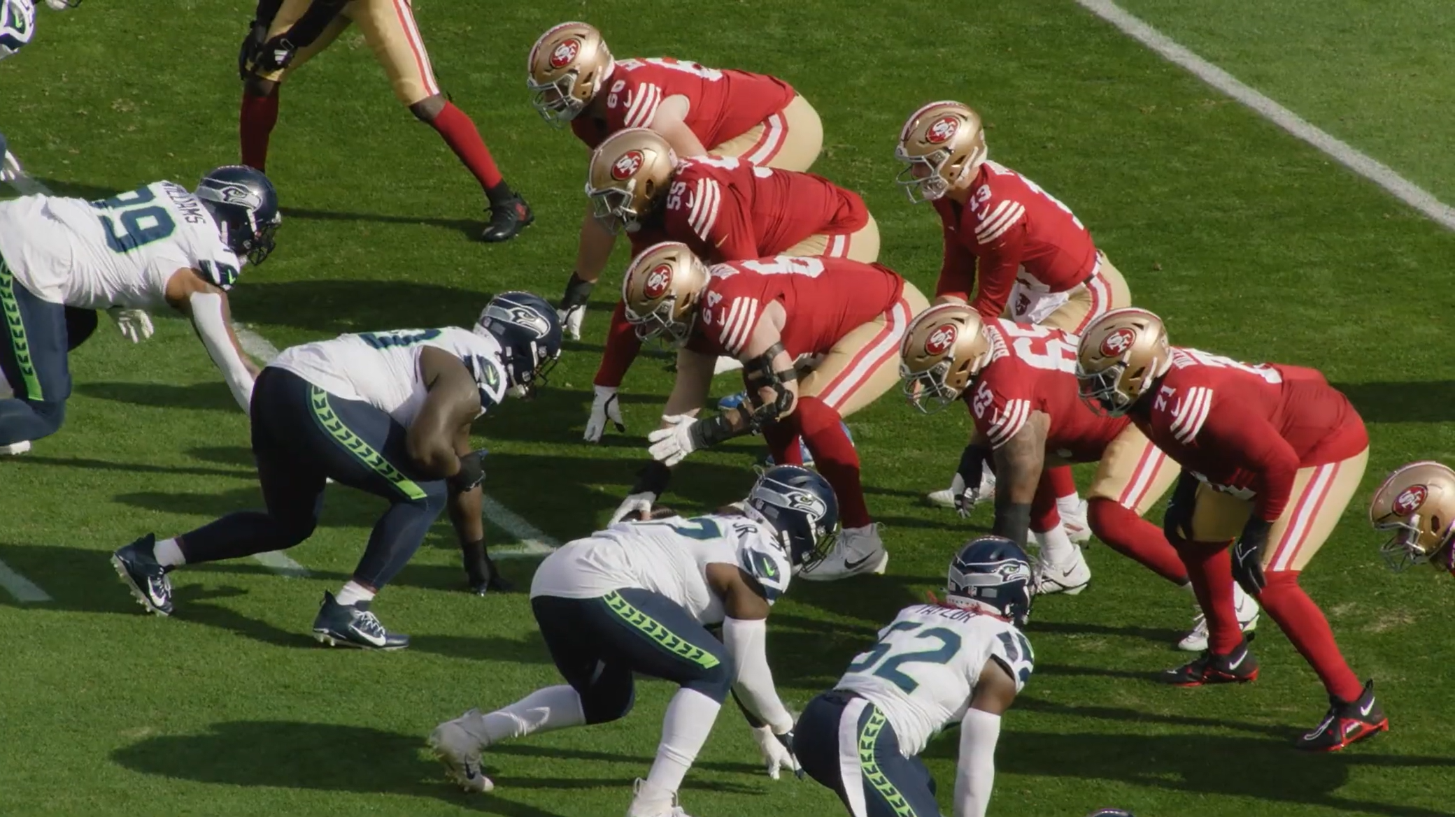
A behind-the-scenes look with the ML Solutions Lab about Coverage Classification, the latest Next Gen Stat from AWS and the NFL, that uses AI to take you inside the huddle to better understand defensive strategies.

ML Solutions Lab: Huan Song, Mohamad Al Jazaery, Haibo Ding, Lin Lee Cheong


1) Give us the main idea behind Coverage Classification and how it came together.

For the last 5 years, AWS and the NFL’s Next Gen Stats team have worked together to put out new advanced stats that showcase specific player skills like fastest ball carriers or decision-based probabilities such as what a coach should do on 4th down. Typically, these metrics have focused on offensive skills players like quarterbacks, running backs, and receivers. But what we’ve been missing to date are the tools to better measure and understand the defensive side of the ball.

What we’ve done here is to use that deep understanding of offense and looked to see what inspiration we could take from that work, and turned our attention to defense. All of these stats we've created over the several years have really been building blocks onto the previous stack. And now in close collaboration with the NFL, we're taking inspiration from what we've learned on the offensive side of the ball to see how defensive analytics can add a new dimension to football analytics and on-field stories.

The objective of Coverage Classification sounds simple but is actually quite complex. The goal is to have an AI-powered system that can distinguish the nuanced differences of and correctly identify defensive coverage schemes on designed pass plays. And do it all in near real-time. These coverage schemes consist of 8 different types in 2 broad categories: cover 0, 1, 2 (these are man coverages, where each defensive player covers certain offensive player), and cover 2, 3, 4, 6, Prevent (these are zone coverages, where each defensive player covers a certain area on the field). 

2) Fans watching a game can pick up visual cues or tendencies to recognize what defense a team is playing. But how do you get a computer to ‘see’ the field and identify different defenses?

This concept of taking what we see with our eyes, combining that with our football knowledge and intuition of identifying defenses, and translating all that into a computer program is incredibly hard.

First, we have to start with the data. We used 60,000 passing plays over the last 4 seasons as our baseline to help us train the AI model. This is based on the NFL’s ability to capture real time location, speed and acceleration data for every player and every play during football games. This is achieved via sensors placed throughout the stadium that track tags placed on players' shoulder pads charting individual movements and the ball.

What makes this data unique is its spatial-temporal nature and the close dependencies between individual players. All players’ movements are closely linked to other players. For example, defense players move by responding to the offense and to the movement of teammates. How this type of interactions progress rapidly over a short period of time is really fascinating.  

But this isn't a straightforward tracking exercise as we need to look carefully at a multitude of information: we need to be able to factor in variables like how defenders line up before the snap, disguising coverages, adjusting to offensive player movement once the ball is snapped, player acceleration, and even blown coverage assignments.

This is one of the reasons why we turned to AI to come up with the right approach. Instead of directly adding complex rules to a computer, we let it learn from large amounts of plays and manually annotated defense labels. We provided the tracking information to the ML model including position, speed, and acceleration. Through the training process as the model tried to emulate the human annotations, it learned to pick up the most important information and develop its internal mechanism to identify the defenses.

Built on AWS SageMaker, it incorporates a custom module to handle complex temporal data, and combines multiple independently trained AI models to handle data and label noise and more. It captures 10 frames per second over the entire offensive play. However, we were able to design the system efficiently so it only needed to use every other frame instead of all the data. 


Figure 1
Figure 1. Raw input tracking data in tabular format. Each row contains the tracking information of a specific timestamp of game for a specific player
3) Can you describe the data pre-processing steps and how this step works?

Raw game tracking data are tabular, as shown in Figure 1. Each row of the table contains a player’s ID, location, speed etc. for a specific timestamp. Data pre-processing transforms the raw tracking data into play samples, where each play is a sequence of frames. We construct each frame as an “image” of features between defense players (“rows”) and offense players (“columns”).

Check out this example play with the raw player positions and the resulting features from the data pre-processing in Figure 2 below. The top figure visualizes the tracking position of each player (annotated by player position) on the field. The bottom figures visualize 4 processed features. At a frame, each pixel of the “image” matrix correspond to a pair of defense and offense players, and the pixel color encodes the value of the feature as annotated by the color-bar. The gif shows movements of the players and how the processed features progress over time. This representation facilitates the modeling of the frame through a CNN.

You can also see that “x position to line of scrimmage” and “x-speed” are defense-only features that do not depend on offense players. And that “relative x position” and “relative x speed” are defense-offense relative features, where each cell in the matrix reflects the feature value for the corresponding player pair. Some examples we can see from the visualization: two defender CBs react to the fast movement of two offense WRs, so their “x speed” and “x position” increase a lot; defender DE closely covers the first offense WR, so their “relative x speed” stays around 0 value. 
Figure 2. GIFs showing the player movement on the field and the temporal progression of 4 features in the defense-offense player matrix format

4) Since this hadn’t been done before, there wasn’t really a playbook to follow. How do you approach building this system?


Starting with the NFL’s goal of being able to correctly identify defenses right after the play occurs, we worked backward from there to build a flexible and efficiency ML system to solve that challenge. But this was not a completely unexplored space as we were inspired by an architecture concept originally submitted by Ben Baldwin during the 2019 Big Data Bowl, which was later replicated by Tom Bliss of the NFL’s Football Operations, to build the foundation of our coverage classification model. And while there are other good modeling techniques developed by the broader football analytics community or other stats, coverage classification is a new task and there are many unique challenges for us to tackle. 

For example, in many plays, there’s not a clear differentiator between one defense versus another, such as when the defense disguises its coverage to deliberately fool the offense or when a defender abandons his assigned coverage. Plus, the coverage schemes are imbalanced: there are a few that called significantly more than others over the course of a game. These factors make distinguishing coverages particularly challenging so we needed to design the architecture to handle these kinds of ambiguities. And in order to advance the technical community, we are sharing lessons of what worked and what didn’t through this building process.

To handle these ambiguities, we used “label smoothing” that adds a bit of uncertainty to the assigned coverage labels during training. We also determined the final architecture of an ensemble of 5 CNN attention models based on experimenting with which techniques improved the baseline model. We trained each of these base models independently from random weights initializations. The final output is the aggregated results among them and we incorporate the average over the results from all base models. Here are some key components that highlight why we chose this approach.

The convolutional neural network (CNN) models each frame as an “image”. Each “pixel” of the image is relative features (relative position, relative speed) between the corresponding pair of defense and offense players. But given that plays are highly dynamic, it’s important to account for the changes over time. We leverage the temporal information of the play in the modeling to make more accurate defensive recognitions. Looking at the frames independently through a CNN alone ended up being insufficient. We utilized an attention model that stacks on top of the CNN and learns what segments of the play to pay attention to. It outperformed the LSTM module from the baseline model and also learned to pay attention and assign more weights to certain key frames. 

5) What data sources did you experiment with to see if it would signficantly improve the model?
 
As part of any experimentation process, there are usually some unexpected outcomes based on things you think will work that don’t and vice versa. Here is a bit more detail on what approaches we explored but ended up not moving ahead with as they did not significantly improve the model.

  • Additional Play Context Features: We already were factoring in a number of different aspects of each play into the model but these were based on player movement. Interested to see if other contextual information from each play would lead to more accurate coverage identifications, we tried incorporating game contextual features including the down, play length, yards to endzone, yards to go, number of pass rushers and number of running routes. In the end, these did not significantly improve the model. Our guess was that the tracking data already contains most game/play information for the model and the contextual features didn’t provide many new things. 
  • Temporal Augmentation: The final model measures information taken from the initial snap to the first 5 seconds of each play. But not all plays take that long and we wanted to find out how that impacted the model’s performance. To test this theory, we added an augmentation that truncates longer plays into short ones, and fed that into the model as additional data. We found that it actually performed worse on shorter plays under 2 seconds in length so did not put this aspect into production.
  • Other Loss Functions: We experimented with other loss functions to train the model. For example, we experimented with “supervised contrastive loss” that tries to put same coverage plays close together and push different coverages apart. But it turned out that the standard cross-entropy loss worked quite well already and the new losses didn’t improve. 

6) You mentioned earlier this importance of taking a ML approach to this, does a computer learn football differently than people?

When people look at the game footage and identify the defense coverages, there’re tons of football knowledge accumulated over time for us to support us making the decision: the football rules, the knowledge of the team, plays and even the coach. The ML model, instead, looks at the tracking data alone, and learns from scratch. It’s remarkable that the model started out knowing nothing about defenses and even about footballs, and learns to recognize them accurately after just a few hours of training. After it has been trained, it takes sub-second recognize the defense.

The early Next Gen Stats relied on solely player tracking data, where we looked at a players’ speed, their acceleration, where they're their orientation of their shoulders, and the direction in which they're running. All of these data points are being streamed to the system, in real time, for every 10th of a second for every player on the field.

One of the more interesting findings we discovered was that a computer doesn't necessarily have to think sequentially like a person does when processing player tracking data. You can imagine that a player goes from Point A to point B to point C to point D during a play. We historically always assumed that that's how to train a ML model to learn what the players are doing on the field. But what we found was a more predictive way to allow the computer to train the model without a specific ordering. Instead, we let the model learn the weights to determine certain points are more important and more predictive than others in determining the actual outcome.

When we inspect the results from the final model, we actually found for some plays, the model identified the correct coverages while the human annotator did not. 

7) Can you give me an example where the ML system was able to more accurately identify a play than a person?

Lets look at this play which was initially labeled a cover 3 zone defense. In this alignment, there are three deep defenders each responsible for defending 1/3 of the field with 4 underneath the deep defenders playing zone. However, our ML model correcly identified that this was man-to-man cover 1 defense.
The most important indicator of coverage classification was that both cornerbacks are lined up close to the receivers at the line of scrimmage and follow them throughout their route as part of their defensive assignments. And with one safety patrolling the middle of the field, that was another indicator leading to the model correctly identifying the defense. One of the reasons this could have been incorrectly labeled is that the other safety and a linebacker follow the tight end and running back when they release from the line of scrimmage following a play-action fake, which makes it harder to tell if these defenders had man coverage responsibilities or not. But when looking at the broader assignments of other on defensive players, it’s safe to assume that the linebackers and safety’s actions are more of a reaction to how the play unfolded than their original assignments.
8) Can you describe the process of working with the NFL’s Next Gen Stats team and how it’s possible to take this kind of research project from the ML Solutions Lab to production where people will see when watching the game? 
 
When setting out to building something entirely new with the NFL, it was important we looked at this challenge from a football and technology standpoint. Meeting frequently with the team, we utilized the Next Gen Stats team’s deep football insight paired with our ML modeling expertise. This helped facilitate comprehensive looks at the challenge and quick turnarounds on the solution development and model iterations.

It’s also important to note that all research and development was done with real-world NFL data. This means it is naturally a ‘noisy’ dataset and all the nuances of capturing data from the game are inherently included. Attempting to retrofit a solution based on a ‘clean’ research dataset would likely not have worked.

We also needed the right tools in place to deliver on this project. AWS SageMaker enabled us to prepare data, and to build and train models easily. Moreover, it’s easy to combine different AWS services to put together a deployment-ready codebase for the NFL.

For example, S3 made it very convenient for us to access the huge amounts of real-world NFL data, and to store and share the intermediate results with NFL from data processing and model training. SageMaker Notebook made prototyping quick and easy for us with the built-in data science/machine learning kernels. It also enables us to access the right amount of computational resources anytime, as we scaled up from playing with a small model and data subset to the full-fledged experimentation through the development process. We used SageMaker Training to quickly trial and error in a short project timespan. We were able to conduct experimentation with multiple development modules in parallel and easily track them to derive improvement and insights. And during the transition, we were able to simply combine these services to hand over to NFL, from data accessing on S3, processing on SageMaker Notebook, to training/inference with SageMaker - it’s all easily streamlined. 
9) We’ve just taken a deep dive into how this was built and why it was a hard engineering challenge to tackle. Zooming back out to a football perspective, why should fans get excited about this new metric?
 
Combined with team and player performance analytics, coverage classification is a foundational metric that will generate several new types on-field stories including how teams and players perform in man vs zone coverage; how teams position their safeties in coverage; how offenses, quarterbacks and receivers perform against different coverage types of the defense team; how often a wide receiver is in man coverage against a cornerback; the relationship between the success of route types against different coverages, and more. By using AI and new, advanced analytics to make these identifications, AWS and the NFL are bringing fans one step closer into the defensive huddle.