Amazon SageMaker は、開発者やデータサイエンティストがあらゆる規模の機械学習モデルを迅速かつ簡単に構築、訓練、およびデプロイすることを可能にする完全マネージド型サービスです。しかし、機械学習 (ML) のワークフローを能率化するだけでなく、Amazon SageMaker は科学技術向けコンピューティングタスクの大規模なスペクトルを実行したり、並列化したりするためのサーバーレスでパワフルな使いやすいコンピューティング環境も提供します。このノートブックでは、TensorFlow と Amazon SageMaker の「bring your own algorithm (BYOA)」 (独自のアルゴリズムを活用する) 機能を併用して、シンプルな量子系をシミュレートする方法についてご紹介します。
この演習を実行するにあたり、Amazon SageMaker にアクセスできる AWS アカウントと Python および TensorFlow に関する基礎知識が必要になります。
量子系の超放射: 簡単な説明
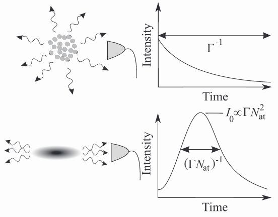
これから私たちがシミュレートする量子効果は超放射として知られています。 これは、ある一定の環境下で、独立した発光体 (個別の原子など) が自然に量子コヒーレンスを増加させ、1 つの実体として協調的に動作するという現象を示します。コヒーレンスが増大したことで、このグループが高輝度のバーストを単発で発します。このバーストは独立した粒子のグループから生じると予想される輝度の N 倍 (!) も強いものである、この場合の N とはグループの粒子の数を示します。興味深いことに、この影響は粒子との相互作用に基づくものではなく、むしろ、粒子の明視野との相互作用と対称的な性質によってのみ生じます。
以下の図では、発光プロファイルが独立型 (上のパネル) と超放射型 (下のパネル) の粒子集団で明確に異なっていることがわかります。超放射は空間的に方向を持った、短時間の高輝度パルスを生じさせます。これは従来の急激に崩壊する放出プロファイルとは異なります。
超放射は多くの様々な量子系で見られ、 提示されてきました。ここでは TensorFlow と Amazon SageMaker を使って、ダイヤモンド窒素-空孔中心の核スピン集団からの超放射をシミュレートする方法を見ていきましょう。
Amazon SageMaker における科学的コンピューティングの構造
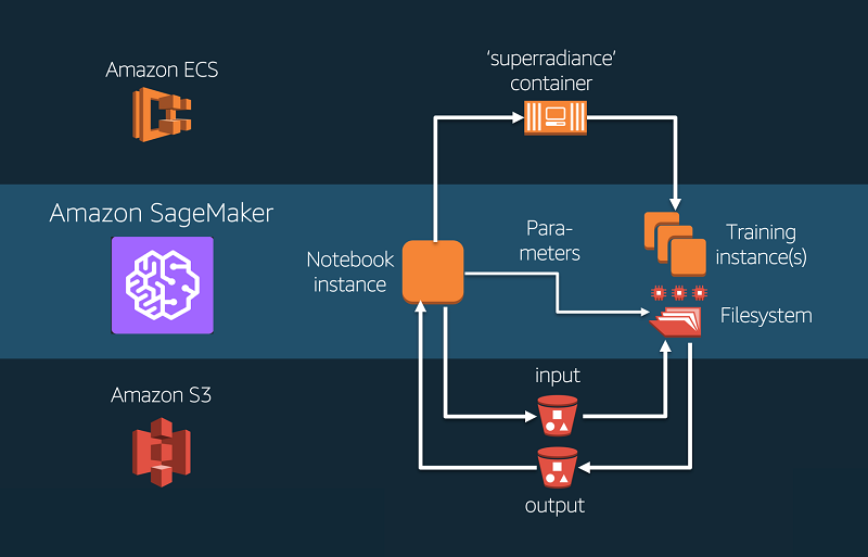
Amazon SageMaker の科学的コンピューティングの中心点がこのノートブックインスタンスです。ここから Jupyter Notebook を使用することで、Amazon SageMaker は科学的ワークロードの様々なステップを連携させるのに役立ちます (次の図を参照)。
ワークロードをコンテナ化する
Amazon SageMaker は Amazon Elastic Container Service (ECS) に、コードの Docker イメージとその従属物 (Python パッケージなど) を送信します。AWS マネジメントコンソールで Amazon ECS コンソールへナビゲートすることにより、過去に自分で送信したイメージにアクセスしたり、それらを管理したりすることができます。
コンピューティング環境を定義しスピンアップする
Amazon SageMaker はトレーニングインスタンスをスピンアップし、コンピューティングを作動させるためにこのブログ記事の前半で定義したコンテナを使用します。 様々なワークロード向けに最適化された多彩なインスタンスタイプから選択できます。クラスター内の複数のインスタンスを使用することで、必要であればコンピューティング環境を並列化できます。
ワークロードの入力データとパラメーターを定義する
シミュレーションに必要な全入力データは、Amazon Simple Storage Service (S3) に格納できます。そこから、Amazon SageMaker はクラスターの各インスタンスでアクセスできてる共有ファイルシステムにデータを転送します。代わりに、Amazon SageMaker のパイプモードを使用して、Amazon S3 から直接データをストリームすることもできます。 より大量のデータをフィードするために S3 を使用する以外では、シミュレーションのパラメーターを直接コンテナに渡すことができます。実際の環境でこれがどのように機能するかについては下記で解説します。
コンピューティングの結果を評価する
コンピューティングが完了したら、Amazon SageMaker はユーザーが選択した Amazon S3 のロケーションに結果を書き込みます。データはここから取得するか、ノートブックで分析できます。
次の図では、Amazon SageMaker の典型的な科学的コンピューティングのワークフローを示しています。まず、Amazon SageMaker はコンテナ化したワークロードを AWS のコンテナレジストリに送信します。次に Amazon SageMaker はユーザーの指定した 1 つまたは複数のコンピューティングインスタンスのクラスターをスピンアップし、ワークロードの含まれるコンテナイメージをロードします。その後、入力データとパラメーターが Amazon S3 から、クラスターの全ノードよりアクセス可能な共有ファイルシステムへ転送されます。計算が完了したら、出力結果はノートブックでさらに分析するため取得可能な場所から Amazon S3 バケットに書き込まれます。 すべてのステップは Amazon SageMaker ノートブックインスタンスから連携させることができます。
設定
皆さんの AWS アカウントでこの例を実行するには、環境のセットアップのためにいくつかのステップを実行する必要があります。
プロセスの中で作成する IAM ロールの名前をメモしておいてください。
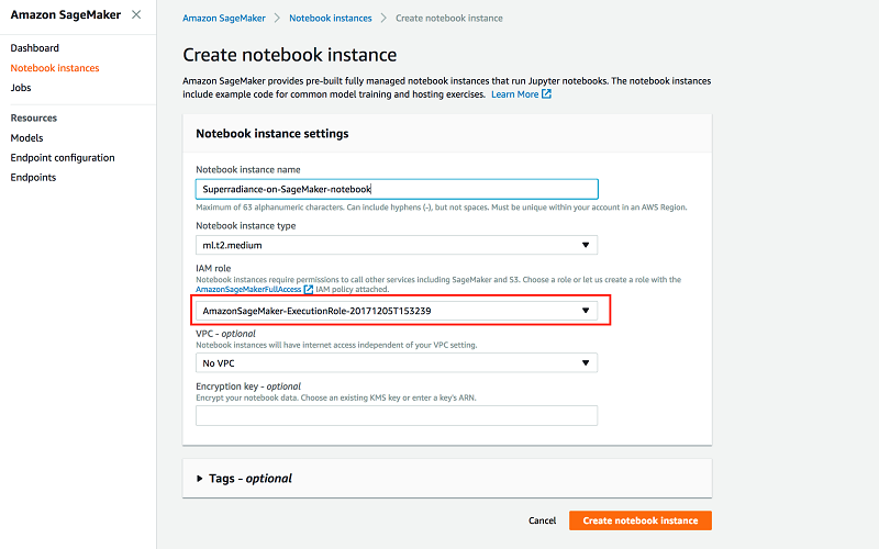
ステップ 1: アクセス許可のセットアップ
始める前に、Amazon ECS へアクセスするための追加アクセス許可を SageMaker ノートブックインスタンスに付与する必要があります。これらのアクセス許可を追加する最も簡単な方法は、SageMaker ダッシュボードでノートブックインスタンスを開始する際に使用したロールにマネージドポリシーを追加する方法です。そのためには、AWS マネジメントコンソールの IAM コンソールへナビゲートし、ロールセクションにアクセスして、Amazon SageMaker ダッシュボードでノートブックインスタンスの開始に使用した SageMaker IAM ロールを見つけます。
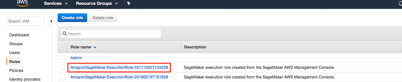
ロールを選択したら、AmazonEC2ContainerRegistryFullAccess ポリシーを接続できます。これを実行する際にノートブックインスタンスを再始動する必要はなく、新しいアクセス権がすぐに使用できるようになります。
ステップ 2: コードリポジトリを SageMaker ノートブックインスタンスにロードする
また、このチュートリアルでこのタスクを実行するには、コードリポジトリを SageMaker ノートブックインスタンスにダウンロードする必要があります。それには Amazon SageMaker でシミュレーションを実行するのに必要な全コンポーネントが含まれ、ユーザー独自のユースケースのテンプレートとして使用できます。
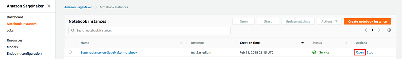
まず、Amazon SageMaker コンソールから SageMaker ノートブックを開きます。
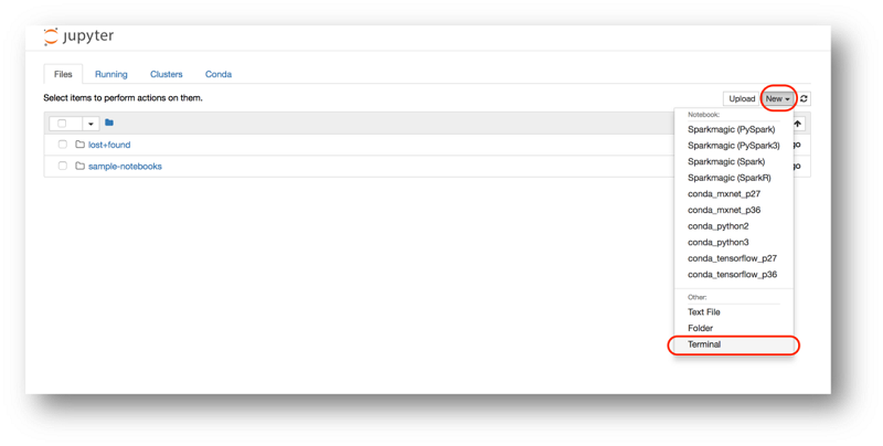
Jupyter ファイルシステムとともに新しいブラウザーのタブが開きます。ターミナルセッションを開くことで、サーバーにログインします。
ターミナルで次のコマンドを使用して、コードリポジトリをダウンロードする
git clone https://github.com/emkessler/sagemaker.git
このリポジトリには Amazon SageMaker のサンプルアルゴリズムをパッケージ化するのに必要な全コンポーネントが入ったコンテナディレクトリが含まれています。個々のコンポーネントについて詳しくは、この SageMaker サンプルノートブックで参照できます。私たちの用途では、最も関連のあるファイルが 2 つあり、ワークロードを実行するための情報がすべて含まれています。
- Dockerfile には Docker コンテナイメージの構築方法が示されています。ここでは、使用する言語 (Python)、コードに必要なパッケージ (TensorFlow など)、その他など、自分のコードの従属物を定義できます。そのほとんどは定型文で、ユーザーのユースケースへの変更に必要であるのは通常、数行のみとなります。詳細については、こちらをご覧ください。
- superradiance/train はコンテナがトレーニング用に実行されるときに呼び出されるプログラムです。 このプログラムにはいくつかのパラメーターとシステムの初期状態がパラメーターとして必要になり、システムのシミュレーションを実行し、numpy 配列として発光プロファイルを返します。この時点ではシミュレーションがどのように機能するかについては心配しないでおきましょう。(シミュレーションについて詳しくは、付録で参照できます。)
ステップ 3: Docker イメージを構築し、プッシュする
Dockerfile から Docker イメージを構築して Amazon ECS にプッシュするには、次のユーティリティスクリプトを実行する必要があります: build_and_push.sh。そのためには、リポジトリに含まれる Jupyter ノートブックを開き、セルで次を実行します。
import subprocess
print subprocess.check_output(['./build_and_push.sh', 'superradiance'])
このスクリプトは superradiance ディレクトリのコードを含む Dockerfile から Docker イメージを構築し、次の名前で Amazon ECS リポジトリへとプッシュします: superradiance (引数は build_and_push.sh に渡されます)。 Amazon -ECS レポジトリが存在しない場合は、自動的に作成されます。
これで、Amazon SageMaker でシミュレーションを実行する準備ができました。
Amazon SageMaker での超放射のシミュレーション
このセクションではいわゆるダイヤモンド窒素-空孔中心から超放射をシミュレートしてみましょう。 窒素空孔中心とは、ダイヤモンドを構成する炭素格子の多数ある潜在的結果の 1 つです。この格子には 2 つの炭素原子が欠けており、そこには空の箇所の隣に窒素原子が 1 つあります。赤いダイヤモンドを見たことはありますか? ほとんどの場合、素材の窒素空孔欠陥が大量にあることが原因でダイヤモンドに色がつきます。ダイヤモンドに美しい色をもたらす (ダイヤモンドの価格を驚く程上げる) ほかに、窒素空孔中心は卓越した量子系にもなります。欠陥の生じた箇所ではエレクトロンが極めて安定した状態で閉じ込められるため、研究者はレーザー光やマイクロ波放射によってこれらのエレクトロンを巧みに操作できるのです。同時に、エレクトロンは電磁力を介して周囲の炭素原子に相互作用をもたらします。そのため、炭素原子の励振がエレクトロンを介して移動し、窒素空孔中心からフォトンとして放出されます。適切な条件下では、この発光は超放射の特性を示します。
まずは、一部のモジュールをインポートし、シミュレーションする時間ステップや炭素原子の数など、シミュレーションのパラメーターを定義するところから始めましょう。
from scipy import sparse
import numpy as np
import os
import pickle
import matplotlib.pyplot as plt

import boto3
from sagemaker import get_execution_role
import sagemaker as sage

steps = 500                  # Number of simulated time steps
N = 8                        # Number of nuclear spins
dim = 2**(N+1)               # Dimension of Hilbert space of N nuclear and 1 electronic spin
8 個の炭素原子と時間ステップ数 500 のシミュレーションを試してみましょう。あとで、これらのパラメーターを次のパラメーター名でプログラムに渡します: hyperparameters。
次に、システムの初期状態を定義します。全炭素原子の時間 t=0 の単純な初期状態からシミュレーションを開始します。また、エレクトロンは電磁的に励起されています。量子力学ではこのような原子とエレクトロンの合成系は、2D 行列、いわゆる密度行列で表示されます。数学の形式主義に深入りしすぎることなく、 物理システムから行列図を引き出すことのできるものによって、幸運なことに、私たちのケースでは、ステートの図は極めて単純です。最初の 3 行でステートを構築したら、Amazon S3 に結果の行列をアップロードします。シミュレーションはこのデータを後で取得し、システムを初期化します。
# Define Nuclear and Electron spin states as density matrices
rhoI = sparse.csr_matrix(([1.],([0],[0])),shape =(int(dim/2),int(dim/2))) # All carbon atoms magnetically excited
rhoS = sparse.csr_matrix(([1.],([1],[1])),shape =(2,2))                   # Electron magnetically excited
sparse_rho =sparse.kron(rhoS, rhoI)                                       # Build the system density matrix

tempfile = '/tmp/tmp.pckl'
pickle.dump(sparse_rho, open(tempfile, "wb"))

# Upload serialized initial state to S3
resource = boto3.resource('s3')
my_bucket = resource.Bucket('sagemaker-kessle31')                         #subsitute this for your s3 bucket name.
my_bucket.upload_file(tempfile, Key='superradiance/initial_state/init.pckl')

# Clean up temporary files
os.remove(tempfile)
これでシミュレーションを積み込む準備が整いました。Docker イメージの指定後、シミュレーションに使用されるハードウェアを定義するトレーニングジョブを作成します。Amazon SageMaker はその後、リクエストされたインスタンスをスピンアップし、Amazon ECS から Docker イメージを引き出して、ジョブを開始します。プログラム (ファイル superradiance/train で定義されたとおり) は TensorFlow を使用して一連の段階的な発展によって、システムの変遷のパターンを説明する連結された微分方程式系を解決します。
role = get_execution_role()
sess = sage.Session()

# Specify the name of the ECS repo that contains your docker image.
# By default the image with tag 'latest' in the repo will be utilized.
imagename = 'superradiance'

account = sess.boto_session.client('sts').get_caller_identity()['Account']
region = sess.boto_session.region_name
image = '{}.dkr.ecr.{}.amazonaws.com/{}'.format(account, region, imagename)

# Define the training job
superradiance = sage.estimator.Estimator(image,
                       role, 1, 'ml.c4.2xlarge',
                       output_path="s3://sagemaker-kessle31/superradiance/output",
                       sagemaker_session=sess)

# Parameters can be passed to the simulation as a dictionary
superradiance.hyperparam_dict = {'N': N, 'steps': steps}

# Pass the location of the training data (see above) and start the job
superradiance.fit("s3://sagemaker-kessle31/superradiance/initial_state")
INFO:sagemaker:Creating training-job with name: superradiance-2018-02-22-16-31-48-732
シミュレーションの結果は、Amazon S3 の次のパスでしてされた場所に、tar.gz ファイルとして出力されます: output_path 引数。さっそく結果を見てみましょう。
import tarfile

# get the results from S3
results = my_bucket.Object('superradiance/output/{}/output/model.tar.gz'.format(superradiance.latest_training_job.name))
tempfile = '/tmp/model.tar.gz'
results.download_file('/tmp/model.tar.gz')

# unzip the results
tar = tarfile.open(tempfile, "r:gz")
tar.extractall(path = '/tmp')

# load the results into the notebook
out = pickle.load(open('/tmp/out.pckl', "rb"))
intensity = out['intensity']
I_ind = out['I_ind']

# clean-up temporary files
os.remove(tempfile)

# Vizualize the results
plt.scatter(range(steps-1),intensity/I_ind, label = 'Simulated System')
plt.scatter(range(steps-1), np.exp(-I_ind/N * np.arange(steps-1)), label = 'Classical System (benchmark)')
plt.xlabel('Time [a.u.]')
plt.ylabel('Intensity of emitted radiation [normalized]')
plt.legend()

plt.show()
以下の図にはシミュレートされた粒子集団 (青) の放出プロファイルが示されています。この放出プロファイルは、従来の集団 (オレンジ) の想定される放出と比較すると、強い輝度のバーストを示しています。
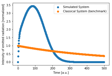
私たちがシミュレーションを行った量子系が、発光プロファイル (青) で特徴的な超放出の兆候を示したことがはっきりと見て取れます。従来の粒子集団 (オレンジ) から想定される放出と比較すると、このプロファイルは超放出を示す短時間後に、強く、独特な爆発的放出を示しています。
まとめ
このブログ記事では、機械学習のワークフローを合理化する手順の他、Amazon SageMaker が一般的な用途や完全なマネージドコンピューティング環境でも利用できることをご覧いただきました。Amazon SageMaker の BYOA 機能を使用して、科学的なワークロードをコンテナ化し、データ入力や出力チャネルの定義、SageMaker クラスターでのワークロードの実行といった様々な方法について学びました。科学的コンピューティングのワークフローでこれらのタスクがすべて 1 つのホストされた Jupyter ノートブックから連携できることをご覧いただきました。
ご不明の点またはご提案があればコメントをお寄せください。
付録: シミュレーションを実行する TensorFlow コード
このブログ記事で実行されたプログラム (superradiance/train) では、シンプルな一連の段階的な発展ごとに、スピンシステムの量子マスター方程式を解くために、TensorFlow を使用しています。主なステップの説明を含むコードを以下に掲載します。
!cat container/superradiance/train
#!/usr/bin/env python

# A sample program that simulates a simple quantum system exhibiting superradiance

from __future__ import print_function
import os
import json
import pickle
import sys
import traceback
import tensorflow as tf
import numpy as np
from utils import kronecker_product, SparseIndices
from scipy import sparse
import pandas as pd

# These are the paths to where SageMaker mounts interesting things in your container.

prefix = '/opt/ml/'

input_path = prefix + 'input/data'

output_path = os.path.join(prefix, 'output')                       # Failure output & error messages should be written here
model_path = os.path.join(prefix, 'model')                         # All results should be written here
param_path = os.path.join(prefix,
                          'input/config/hyperparameters.json')     # Passed parameters can be retrieved here

# This algorithm has a single channel of input data called 'training'. Since we run in
# File mode, the input files are copied to the directory specified here.
channel_name='training'
training_path = os.path.join(input_path, channel_name)              # The initial state is found here


# The function to execute the training.
def train():
    print('Starting the training.')
    try:
        ##################################################################################
        # Retrieve parameters
        ##################################################################################
        # Parameters that were defined in the hyperparameter dict in the notebook
        # (in our example: superradiance.hyperparam_dict = {'N': N, 'steps': steps})
        # can be retrieved from the param_path defined above.
        # Note that the parameters are stored as a JSON string, so it is required to
        # define the correct dtype upon reading (here: int).

        datatype = tf.complex128

        with open(param_path, 'r') as tc:
             trainingParams = json.load(tc)
        N = int(trainingParams.get('N', None))          # Number of simulated nuclear spins as defined in notebook
        steps = int(trainingParams.get('steps', None))  # Number of simulated time steps

        dim = 2**(N+1)                                  # Dimension of Hilbert space of N nuclear and 1 electronic spin

        #################################################################################
        # Define some other parameters
        ##################################################################################

        Amean = 1
        gamma = 1
        #g = np.random.randn(N)
        g = np.ones(N)
        g = g/(np.sqrt((g**2).sum()))                    # Coupling strengts
        A = Amean/g.sum()
        I_ind = np.real(A**2/(gamma+1j*Amean))*2/N       # Classical emission intensity of N independent emitters (benchmark)

        ##################################################################################
        # Define TF constants
        ##################################################################################

        gammaT = tf.constant(gamma, dtype=datatype)
        AT = tf.constant(A, dtype=datatype)
        eps = tf.placeholder(dtype=datatype, shape=())

        ##################################################################################
        # Define 'Pauli Matrices'
        ##################################################################################
        # The most elemental quantum mechanical spins system is a spin-1/2. It can be
        # represented through three simple matrices, called Pauli Matrices. For more
        # information, there are many great online resources, e.g.,
        # http://galileo.phys.virginia.edu/~pf7a/msm3.pdf

        sigmaz = tf.constant([[1/2, 0], [0, -1/2]], dtype= datatype)
        splus  = tf.constant([[0, 1], [0, 0]], dtype = datatype)
        sminus = tf.constant([[0, 0], [1, 0]], dtype = datatype)

        ##################################################################################
        # Electron Spin operators
        ##################################################################################
        # States of a quantum system live in a vector space with special properties,
        # called the Hilbert space.
        # The Hilbert space of a composite system of multiple spins can be constructed by
        # taking the tensor product of the individual 1-particle spaces.
        # Using this property, it can be shown that we can construct the multi-spin
        # operators by taking the the Kronecker product (https://en.wikipedia.org/wiki/Kronecker_product)
        # of the individual spin operators with the identity matrix of appropriate dimension
        # (see, section 3.2 of http://galileo.phys.virginia.edu/~pf7a/msm3.pdf)
        # Let's see how that looks like for our electron operator:

        Sm = kronecker_product(sminus, tf.eye(int(dim/2), dtype = datatype))
        Sp = tf.transpose(Sm)
        Sz = kronecker_product(sigmaz, tf.eye(int(dim/2), dtype = datatype))

        ##################################################################################
        # Nuclear Spin operators
        ##################################################################################
        # Similarly to the case of the electron operator, we create one spin operator
        # for every nuclear spin we simulate, and take the sum over all nuclear operators
        # (because the electron interacts with all of them)

        Am = tf.zeros(int(dim/2), dtype = datatype)
        Iz = tf.zeros(int(dim/2), dtype = datatype)
        for p in range(N):
            Am = Am + g[p]*kronecker_product(kronecker_product(tf.eye(2**p, dtype = datatype),sminus)
                                           ,tf.eye(2**(N-1-p), dtype = datatype))
            Iz = Iz +      kronecker_product(kronecker_product(tf.eye(2**p, dtype = datatype),sigmaz)
                                           ,tf.eye(2**(N-1-p), dtype = datatype))

        Am = kronecker_product(tf.eye(2, dtype = datatype),Am)
        Ap = tf.transpose(Am)
        Iz = kronecker_product(tf.eye(2, dtype = datatype),Iz)

        ##################################################################################
        # Load and construct Initial State
        ##################################################################################
        # You can pass on larger data structures to your program by placing them on S3 and
        # and point to the location at execution time.
        # (in our example: superradiance.fit("s3://sagemaker-kessle31/superradiance/initial_state")
        # It can be retrieved from the 'training_path' location defined above.

        sparse_rho = pickle.load(open(os.path.join(training_path, 'init.pckl'), "rb"))

        rho_ind = SparseIndices(sparse_rho)
        rho2 = tf.sparse_to_dense(rho_ind['indices'],
                                  rho_ind['dense_shape'],
                                  rho_ind['values'])         # Sparse_to_dense not implemented for complex at time of this
                                                             # notebook => Construct Real an Imag separately
        rho1 = tf.complex(rho2,tf.zeros(rho_ind['dense_shape'], dtype=tf.float64))
        rho = tf.Variable(rho1, dtype=datatype)

        ##################################################################################
        # Define Operations
        ##################################################################################
        # The Hamiltonian and Lagrangian are operators codifying the dynamics and interactions
        # of a Quantum System.
        # The system we are simulating is a simple central spin system represented by the
        # following Hamiltonian/Lagrangian:
        # (https://journals.aps.org/prl/abstract/10.1103/PhysRevLett.104.143601)

        H = 0.5 * AT * (tf.matmul(Sp,Am) + tf.matmul(Sm,Ap))  # Define the Hamiltonian of the system

        IL = gammaT*(tf.matmul(tf.matmul(Sm,rho),Sp)
                     - 0.5 * (tf.matmul(tf.matmul(Sp,Sm),rho)
                              + tf.matmul(rho, tf.matmul(Sp,Sm))))\
              - 1j * (tf.matmul(H,rho) - tf.matmul(rho, H))   # Define the Lagrangian of the system

        rho_ = rho + eps * IL                                 # Evolve the system by one time step

        pol = tf.real(tf.trace(tf.matmul(rho, Iz)))           # Compute the polarization of the nuclear system,

        global_step = tf.train.get_or_create_global_step()
        increment_global_step_op = tf.assign(global_step, global_step+1)

        step = tf.group(rho.assign(rho_),increment_global_step_op)

        ##################################################################################
        # Run the Simulation
        ##################################################################################

        polarization = np.zeros(steps)
        init = tf.global_variables_initializer()
        with tf.Session() as sess:
            sess.run(init)
            for i in range(steps):
                _ , polarization[i] = sess.run([step, pol], feed_dict={eps:0.3})

        ##################################################################################
        # Compute output and dump to pickle
        ##################################################################################
        # Everything written into the 'model_path' location defined above will be
        # returned by SageMaker to the S3 location defined in the notebook
        # (in our example: output_path="s3://sagemaker-kessle31/superradiance/output")
        # Note that the files will be returned as a tar.gz archive

        intensity = -np.diff(polarization)
        out= {'intensity': intensity, 'I_ind': I_ind}
        pickle.dump(out, open(os.path.join(model_path, 'out.pckl'), "wb"))

        print('Training complete.')

    except Exception as e:
        # Write out an error file. This will be returned as the failureReason in the
        # DescribeTrainingJob result.
        trc = traceback.format_exc()
        with open(os.path.join(output_path, 'failure'), 'w') as s:
            s.write('Exception during training: ' + str(e) + '\n' + trc)
        # Printing this causes the exception to be in the training job logs, as well.
        print('Exception during training: ' + str(e) + '\n' + trc, file=sys.stderr)
        # A non-zero exit code causes the training job to be marked as Failed.
        sys.exit(255)

if __name__ == '__main__':
    train()

    # A zero exit code causes the job to be marked a Succeeded.
    sys.exit(0)
今回のブログ投稿者について
 Eric Kessler は AWS プロフェッショナルサービスのデータサイエンティストです。 彼はドイツのマックスプランク量子光学研究所にて博士号を取得し、数年間、量子物理学の学術研究者として働いていました。現在は、AWS の機械学習と AI ソリューションの開発および統合のために、お客様と協業しています。