Amazon SageMaker Processingによるシフトスケジュール、輸送経路選択、資源配分などの数理最適化問題の解決

この記事では、 Amazon SageMaker Processing API を使用して数値最適化問題を解く方法について説明します。最適化とは、様々な制約条件のもと、ある関数の最小値（または最大値）を求めるプロセスです。このパターンは、作業スタッフのシフト作成や輸送ルート選定、在庫配分、形状や軌跡の最適化など、ビジネスにおける重要な問題の解決に役立ちます。このような問題を解くためには、商用もしくはオープンソースで提供される“ソルバー”というソフトウェアが利用されます。この記事では、無償で利用できる3つの一般的な Python のソルバーを SageMaker Processingで実行し、これらの最適化問題を解く方法を示します。

概要

SageMaker Processing により、データサイエンティストと ML エンジニアは、SageMaker 上で前処理や後処理、モデル評価などのAIや機械学習に必要なタスクを簡単に実行できるようになります。このSDKは、scikit-learn と Spark の組み込みコンテナを使用しますが、独自の Docker イメージを使用することもできます。これにより、SageMaker Processing に限らず、Amazon Elastic Container Service (Amazon ECS) や Amazon Elastic Kubernetes Service (Amazon EKS) のようなAWSコンテナサービス、あるいはオンプレミスであっても、どんなコードも実行できるという柔軟性が得られます。まず、一般的な最適化パッケージとソルバーを含んだ Docker イメージをビルドし、以下の3つの最適化例題を解きます。

物流ネットワークを通じて商品を出荷するコストを最小化する
病院における看護師のシフトをスケジューリングする
アポロ11号の月着陸船を最小の燃料で着陸させる軌道を求める

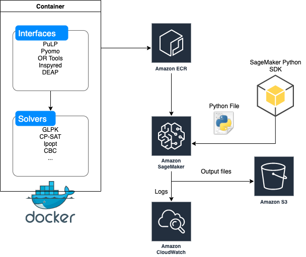
それぞれの例題を、対応するソルバーを使用して解きます。おおまかには以下のステップに沿って各例題を解決します（こちらのノートブックを参照）。

最適化ソルバー（GLPK や CBC など）に対応する Python インターフェース（Pyomo や PuLP など）を含む Docker コンテナのイメージをビルドする。
Amazon Elastic Container Registry (Amazon ECR) のリポジトリにビルドしたコンテナイメージをプッシュする。
SageMaker Python SDKを使用して（ノートブックなどから）Amazon ECRの Docker イメージを指定し、実際の最適化問題のコードを含むPythonファイルを送信します。
ノートブックまたは Amazon CloudWatch Logs でログを監視し、指定した Amazon Simple Storage Service（Amazon S3）の出力フォルダで結果を取得します。

以下にこの処理の全体像を図解します。

それでは始めましょう。

DockerコンテナのビルドとECRへのプッシュ

まずは以下のような Docker ファイルを作成します。

FROM continuumio/anaconda3
RUN pip install boto3 pandas scikit-learn pulp pyomo inspyred ortools scipy deap
RUN conda install -c conda-forge ipopt coincbc glpk
ENV PYTHONUNBUFFERED=TRUE
ENTRYPOINT ["python"]

このコードでは、ソルバーにアクセスする Python インタフェースをインストールしています。ソルバーとは PuLP や Pyomo、Inspyred、OR-Tools、Scipy、DEAP のようなソフトウェアです。これらソルバーについてのより詳細な情報は、この記事の最後にある参考情報のセクションを参考にしてください。

以下のコードをノートブックから実行することで、コンテナイメージがビルドされ、Amazon ECR にプッシュされます。

import boto3

account_id = boto3.client('sts').get_caller_identity().get('Account')
ecr_repository = 'sagemaker-opt-container'
tag = ':latest'
processing_repository_uri = '{}.dkr.ecr.{}.amazonaws.com/{}'.format(account_id, region, ecr_repository + tag)

# Create ECR repository and push docker image
!docker build -t $ecr_repository docker
!$(aws ecr get-login --region $region --registry-ids $account_id --no-include-email)
!aws ecr create-repository --repository-name $ecr_repository
!docker tag {ecr_repository + tag} $processing_repository_uri
!docker push $processing_repository_uri

上記のコードを実行した結果、以下のような出力が得られます（出力結果はサンプルであるため実行環境によって異なる点にご注意ください）。

Sending build context to Docker daemon  2.048kB
Step 1/5 : FROM continuumio/anaconda3
 ---> bbf09a95b565
Step 2/5 : RUN pip install boto3 pandas scikit-learn pulp pyomo inspyred ortools scipy deap
 ---> Using cache
 ---> 90655e74a46d
Step 3/5 : RUN conda install -c conda-forge ipopt coincbc glpk
 ---> Using cache
 ---> d61d5542b339
Step 4/5 : ENV PYTHONUNBUFFERED=TRUE
 ---> Using cache
 ---> 56636836f8ae
Step 5/5 : ENTRYPOINT ["python"]
 ---> Using cache
 ---> f3e5b0f6e957
Successfully built f3e5b0f6e957
Successfully tagged sagemaker-opt-container:latest
WARNING! Using --password via the CLI is insecure. Use --password-stdin.
WARNING! Your password will be stored unencrypted in /home/ec2-user/.docker/config.json.
Configure a credential helper to remove this warning. See
https://docs.docker.com/engine/reference/commandline/login/#credentials-store

Login Succeeded
{
    "repository": {
        "repositoryArn": "arn:aws:ecr:us-east-2:xxxxxxxxxxxx:repository/sagemaker-opt-container",
        "registryId": "xxxxxxxxxxxx",
        "repositoryName": "sagemaker-opt-container",
        "repositoryUri": "xxxxxxxxxxxx.dkr.ecr.us-east-2.amazonaws.com/sagemaker-opt-container",
        "createdAt": 1691281443.0,
        "imageTagMutability": "MUTABLE",
        "imageScanningConfiguration": {
            "scanOnPush": false
        },
        "encryptionConfiguration": {
            "encryptionType": "AES256"
        }
    }
}
The push refers to repository [xxxxxxxxxx.dkr.ecr.us-east-2.amazonaws.com/sagemaker-opt-container]

689828f5: Preparing 
7ca1d711: Preparing 
8bbb3a9d: Preparing 
8bbb3a9d: Pushing  2.302GB/4.828GBPushing  1.843GB/4.828GB
8bbb3a9d: Pushed   4.954GB/4.828GBPushing  2.811GB/4.828GBPushing  3.629GB/4.828GBPushing  3.851GB/4.828GBPushing  3.973GB/4.828GBPushing   4.42GB/4.828GBPushing  4.437GB/4.828GBPushing  4.531GB/4.828GBlatest: digest: sha256:428c97609616197615e370da1f78b3aefaebd9ae7ac7739bad0ecb7849512cd1 size: 1169

SageMaker Python SDKによるジョブの実行

まず、以下のように SageMaker ProcessingScriptProcessorを初期化します。

script_processor = ScriptProcessor(command=['python'],
                image_uri=processing_repository_uri,
                role=role,
                instance_count=1,
                instance_type='ml.m5.xlarge')

そして、スクリプトファイル(この記事では“preprocessing.py”というファイル名で作成します)を記述し、以下のように SageMaker の Processingジョブを実行します。

from sagemaker.processing import ProcessingInput, ProcessingOutput

script_processor.run(code='preprocessing.py',
                      outputs=[ProcessingOutput(output_name='data',
                                                source='/opt/ml/processing/data')])

script_processor_job_description = script_processor.jobs[-1].describe()
print(script_processor_job_description)

例題1: 最小のコストで商品を配送する流通ネットワークを選択する

オハイオ州に拠点を置く鋼鉄製造会社であるAmerican Steel社は、ヤングスタウンとピッツバーグにある2つの製鉄所で鋼鉄を生産しています。同社は地域倉庫と現場倉庫で構成される流通ネットワークを通じて、完成品の鋼鉄を小売り顧客に供給しています。
このネットワークでは、American Steel社の2つの製鉄所ヤングスタウン（ノード1）とピッツバーグ（ノード2）で製造された鋼鉄が、現場倉庫であるオールバニ、ヒューストン、テンペ、ゲーリー（ノード6、7、8、9）へ出荷されます。ただしその途中で、シンシナティ、カンザスシティ、シカゴ（ノード3、4、5）の3つの地域倉庫を経由します。なお、一部の現場倉庫へは製鉄所から直接製品が供給されることもあります。
以下の表は、それぞれの都市間で輸送可能な鋼鉄の最小および最大量と、1,000トンあたり1ヶ月の鋼鉄の輸送コストを示しています。例えば、ヤングスタウンからカンザスシティへの出荷は鉄道会社によって行われますが、最小出荷量が1,000トン/月の契約を結んでいます。ただし、鉄道会社の車両数の制限により1ヶ月に5,000トン以上を出荷することができません。

発地	着地	コスト	最小輸送量/月	最大輸送量/月
Youngstown	Albany	500	–	1000
Youngstown	Cincinnati	350	–	3000
Youngstown	Kansas City	450	1000	5000
Youngstown	Chicago	375	–	5000
Pittsburgh	Cincinnati	350	–	2000
Pittsburgh	Kansas City	450	2000	3000
Pittsburgh	Chicago	400	–	4000
Pittsburgh	Gary	450	–	2000
Cincinnati	Albany	350	1000	5000
Cincinnati	Houston	550	–	6000
Kansas City	Houston	375	–	4000
Kansas City	Tempe	650	–	4000
Chicago	Tempe	600	–	2000
Chicago	Gary	120	–	4000

一般的な転送問題と同様、American Steel社の目的はネットワークを通じて商品を出荷するコストを最小限にすることです。
本例題では、次の流入保存制約に従う必要があります。製品を製造する”製鉄所“には「供給」が定義されており、ここから流出する商品は「供給」量以下である必要があります。また、消費地に近い”現場倉庫“には「需要」が定義されており、「需要」量以上の商品が流入される必要があります。また、各ノードへの流入量は流出量以上である必要があります。
この問題は以下のようにコード化されます。

%%writefile preprocessing.py

import argparse
import os
import warnings

"""
The American Steel Problem for the PuLP Modeller

Authors: Antony Phillips, Dr Stuart Mitchell  2007
"""

# Import PuLP modeller functions
from pulp import *

# List of all the nodes
Nodes = ["Youngstown",
         "Pittsburgh",
         "Cincinatti",
         "Kansas City",
         "Chicago",
         "Albany",
         "Houston",
         "Tempe",
         "Gary"]

nodeData = {# NODE        Supply Demand
         "Youngstown":    [10000,0],
         "Pittsburgh":    [15000,0],
         "Cincinatti":    [0,0],
         "Kansas City":   [0,0],
         "Chicago":       [0,0],
         "Albany":        [0,3000],
         "Houston":       [0,7000],
         "Tempe":         [0,4000],
         "Gary":          [0,6000]}

# List of all the arcs
Arcs = [("Youngstown","Albany"),
        ("Youngstown","Cincinatti"),
        ("Youngstown","Kansas City"),
        ("Youngstown","Chicago"),
        ("Pittsburgh","Cincinatti"),
        ("Pittsburgh","Kansas City"),
        ("Pittsburgh","Chicago"),
        ("Pittsburgh","Gary"),
        ("Cincinatti","Albany"),
        ("Cincinatti","Houston"),
        ("Kansas City","Houston"),
        ("Kansas City","Tempe"),
        ("Chicago","Tempe"),
        ("Chicago","Gary")]

arcData = { #      ARC                Cost Min Max
        ("Youngstown","Albany"):      [0.5,0,1000],
        ("Youngstown","Cincinatti"):  [0.35,0,3000],
        ("Youngstown","Kansas City"): [0.45,1000,5000],
        ("Youngstown","Chicago"):     [0.375,0,5000],
        ("Pittsburgh","Cincinatti"):  [0.35,0,2000],
        ("Pittsburgh","Kansas City"): [0.45,2000,3000],
        ("Pittsburgh","Chicago"):     [0.4,0,4000],
        ("Pittsburgh","Gary"):        [0.45,0,2000],
        ("Cincinatti","Albany"):      [0.35,1000,5000],
        ("Cincinatti","Houston"):     [0.55,0,6000],
        ("Kansas City","Houston"):    [0.375,0,4000],
        ("Kansas City","Tempe"):      [0.65,0,4000],
        ("Chicago","Tempe"):          [0.6,0,2000],
        ("Chicago","Gary"):           [0.12,0,4000]}

# Splits the dictionaries to be more understandable
(supply, demand) = splitDict(nodeData)
(costs, mins, maxs) = splitDict(arcData)

# Creates the boundless Variables as Integers
vars = LpVariable.dicts("Route",Arcs,None,None,LpInteger)

# Creates the upper and lower bounds on the variables
for a in Arcs:
    vars[a].bounds(mins[a], maxs[a])

# Creates the 'prob' variable to contain the problem data    
prob = LpProblem("American Steel Problem",LpMinimize)

# Creates the objective function
prob += lpSum([vars[a]* costs[a] for a in Arcs]), "Total Cost of Transport"

# Creates all problem constraints - this ensures the amount going into each node is at least equal to the amount leaving
for n in Nodes:
    prob += (supply[n]+ lpSum([vars[(i,j)] for (i,j) in Arcs if j == n]) >=
             demand[n]+ lpSum([vars[(i,j)] for (i,j) in Arcs if i == n])), "Steel Flow Conservation in Node %s"%n

# The problem data is written to an .lp file
prob.writeLP('/opt/ml/processing/data/' + 'AmericanSteelProblem.lp')

# The problem is solved using PuLP's choice of Solver
prob.solve()

# The status of the solution is printed to the screen
print("Status:", LpStatus[prob.status])

# Each of the variables is printed with it's resolved optimum value
for v in prob.variables():
    print(v.name, "=", v.varValue)

# The optimised objective function value is printed to the screen    
print("Total Cost of Transportation = ", value(prob.objective))

この例題を PuLP とそのデフォルトのソルバーである CBC を script_processor.run で実行します。この最適化ジョブは以下のログを出力します。

Status: Optimal
Route_('Chicago',_'Gary') = 4000.0
Route_('Chicago',_'Tempe') = 2000.0
Route_('Cincinatti',_'Albany') = 2000.0
Route_('Cincinatti',_'Houston') = 3000.0
Route_('Kansas_City',_'Houston') = 4000.0
Route_('Kansas_City',_'Tempe') = 2000.0
Route_('Pittsburgh',_'Chicago') = 3000.0
Route_('Pittsburgh',_'Cincinatti') = 2000.0
Route_('Pittsburgh',_'Gary') = 2000.0
Route_('Pittsburgh',_'Kansas_City') = 3000.0
Route_('Youngstown',_'Albany') = 1000.0
Route_('Youngstown',_'Chicago') = 3000.0
Route_('Youngstown',_'Cincinatti') = 3000.0
Route_('Youngstown',_'Kansas_City') = 3000.0
Total Cost of Transportation =  15005.0

例題2: 病院における看護師のシフトをスケジューリングする（ナーススケジューリング）

この例題では、4人の看護師の3日間の勤務スケジュールを作成します。ただし、勤務表の作成にあたっては以下の条件を満たす必要があります。

1日のスケジュールは 8 時間の 3 つのシフトで構成されます。
1日の中で 1 人の看護師が割り当てられるシフトは1つです。複数のシフトを勤務することはできません。
各看護師は 3 日間の期間中に少なくとも 2 つのシフトに割り当てられます。

このスケジューリング問題についてさらに詳しい情報はこちらをご参照ください。
この例題は以下のようにコード化されます。

%%writefile preprocessing.py

from __future__ import print_function
from ortools.sat.python import cp_model

class NursesPartialSolutionPrinter(cp_model.CpSolverSolutionCallback):
    """Print intermediate solutions."""

    def __init__(self, shifts, num_nurses, num_days, num_shifts, sols):
        cp_model.CpSolverSolutionCallback.__init__(self)
        self._shifts = shifts
        self._num_nurses = num_nurses
        self._num_days = num_days
        self._num_shifts = num_shifts
        self._solutions = set(sols)
        self._solution_count = 0

    def on_solution_callback(self):
        if self._solution_count in self._solutions:
            print('Solution %i' % self._solution_count)
            for d in range(self._num_days):
                print('Day %i' % d)
                for n in range(self._num_nurses):
                    is_working = False
                    for s in range(self._num_shifts):
                        if self.Value(self._shifts[(n, d, s)]):
                            is_working = True
                            print('  Nurse %i works shift %i' % (n, s))
                    if not is_working:
                        print('  Nurse {} does not work'.format(n))
            print()
        self._solution_count += 1

    def solution_count(self):
        return self._solution_count

def main():
    # Data.
    num_nurses = 4
    num_shifts = 3
    num_days = 3
    all_nurses = range(num_nurses)
    all_shifts = range(num_shifts)
    all_days = range(num_days)
    # Creates the model.
    model = cp_model.CpModel()

    # Creates shift variables.
    # shifts[(n, d, s)]: nurse 'n' works shift 's' on day 'd'.
    shifts = {}
    for n in all_nurses:
        for d in all_days:
            for s in all_shifts:
                shifts[(n, d,
                        s)] = model.NewBoolVar('shift_n%id%is%i' % (n, d, s))

    # Each shift is assigned to exactly one nurse in the schedule period.
    for d in all_days:
        for s in all_shifts:
            model.Add(sum(shifts[(n, d, s)] for n in all_nurses) == 1)

    # Each nurse works at most one shift per day.
    for n in all_nurses:
        for d in all_days:
            model.Add(sum(shifts[(n, d, s)] for s in all_shifts) <= 1)

    # min_shifts_per_nurse is the largest integer such that every nurse
    # can be assigned at least that many shifts. If the number of nurses doesn't
    # divide the total number of shifts over the schedule period,
    # some nurses have to work one more shift, for a total of
    # min_shifts_per_nurse + 1.
    min_shifts_per_nurse = (num_shifts * num_days) // num_nurses
    max_shifts_per_nurse = min_shifts_per_nurse + 1
    for n in all_nurses:
        num_shifts_worked = sum(
            shifts[(n, d, s)] for d in all_days for s in all_shifts)
        model.Add(min_shifts_per_nurse <= num_shifts_worked)
        model.Add(num_shifts_worked <= max_shifts_per_nurse)

    # Creates the solver and solve.
    solver = cp_model.CpSolver()
    solver.parameters.linearization_level = 0
    # Display the first five solutions.
    a_few_solutions = range(5)
    solution_printer = NursesPartialSolutionPrinter(shifts, num_nurses,
                                                    num_days, num_shifts,
                                                    a_few_solutions)
    solver.SearchForAllSolutions(model, solution_printer)

    # Statistics.
    print()
    print('Statistics')
    print('  - conflicts       : %i' % solver.NumConflicts())
    print('  - branches        : %i' % solver.NumBranches())
    print('  - wall time       : %f s' % solver.WallTime())
    print('  - solutions found : %i' % solution_printer.solution_count())


if __name__ == '__main__':
    main()

この例題を OR-Tools とソルバーのCP-SATを使うよう、script_processor.run で実行します。この最適化ジョブは以下のログを出力します。

Solution 0
Day 0
  Nurse 0 does not work
  Nurse 1 works shift 0
  Nurse 2 works shift 1
  Nurse 3 works shift 2
Day 1
  Nurse 0 works shift 2
  Nurse 1 does not work
  Nurse 2 works shift 1
  Nurse 3 works shift 0
Day 2
  Nurse 0 works shift 2
  Nurse 1 works shift 1
  Nurse 2 works shift 0
  Nurse 3 does not work

Solution 1
Day 0
  Nurse 0 works shift 0
  Nurse 1 does not work
  Nurse 2 works shift 1
  Nurse 3 works shift 2
Day 1
  Nurse 0 does not work
  Nurse 1 works shift 2
  Nurse 2 works shift 1
  Nurse 3 works shift 0
Day 2
  Nurse 0 works shift 2
  Nurse 1 works shift 1
  Nurse 2 works shift 0
  Nurse 3 does not work

Solution 2
Day 0
  Nurse 0 works shift 0
  Nurse 1 does not work
  Nurse 2 works shift 1
  Nurse 3 works shift 2
Day 1
  Nurse 0 works shift 1
  Nurse 1 works shift 2
  Nurse 2 does not work
  Nurse 3 works shift 0
Day 2
  Nurse 0 works shift 2
  Nurse 1 works shift 1
  Nurse 2 works shift 0
  Nurse 3 does not work

Solution 3
Day 0
  Nurse 0 works shift 0
  Nurse 1 does not work
  Nurse 2 works shift 1
  Nurse 3 works shift 2
Day 1
  Nurse 0 works shift 2
  Nurse 1 works shift 1
  Nurse 2 does not work
  Nurse 3 works shift 0
Day 2
  Nurse 0 works shift 2
  Nurse 1 works shift 1
  Nurse 2 works shift 0
  Nurse 3 does not work

Solution 4
Day 0
  Nurse 0 does not work
  Nurse 1 works shift 0
  Nurse 2 works shift 1
  Nurse 3 works shift 2
Day 1
  Nurse 0 works shift 2
  Nurse 1 works shift 1
  Nurse 2 does not work
  Nurse 3 works shift 0
Day 2
  Nurse 0 works shift 2
  Nurse 1 works shift 1
  Nurse 2 works shift 0
  Nurse 3 does not work


Statistics
  - conflicts       : 37
  - branches        : 41231
  - wall time       : 0.367511 s
  - solutions found : 5184

例題3: アポロ11号の月着陸船を最小の燃料で着陸させる軌道を求める

この例題では、 Pyomo によるシンプルな宇宙ロケットのモデルを使用して、月面着陸のための制御ポリシーを計算します。
ここで使用しているパラメータは、1969年7月20日のアポロ11号月着陸船の月への降下時のものです。高度 h で垂直飛行中の質量 m のロケットの場合、運動量バランスにより次のモデルが得られます。

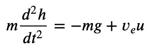
このモデルでは、 u は推進剤の質量流量、ve はロケットに対する排気の速度を表しています。モデリングと制御のこの最初の試みでは、燃料の燃焼によるロケットの質量の変化を無視します。
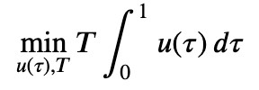
燃料消費量は以下の式で算出されます。

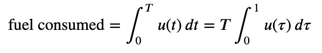
さらに以下で燃料消費量が最小となるような軌道を求めます。

この例題は以下のようにコード化されます。

%%writefile preprocessing.py

import numpy as np

from pyomo.environ import *
from pyomo.dae import *

#Define constants ...
# lunar module
m_ascent_dry = 2445.0          # kg mass of ascent stage without fuel
m_ascent_fuel = 2376.0         # kg mass of ascent stage fuel
m_descent_dry = 2034.0         # kg mass of descent stage without fuel
m_descent_fuel = 8248.0        # kg mass of descent stage fuel

m_fuel = m_descent_fuel
m_dry = m_ascent_dry + m_ascent_fuel + m_descent_dry
m_total = m_dry + m_fuel

# descent engine characteristics
v_exhaust = 3050.0             # m/s
u_max = 45050.0/v_exhaust      # 45050 newtons / exhaust velocity

# landing mission specifications
h_initial = 100000.0           # meters
v_initial = 1520               # orbital velocity m/s
g = 1.62                       # m/s**2

m = ConcreteModel()
m.t = ContinuousSet(bounds=(0, 1))
m.h = Var(m.t)
m.u = Var(m.t, bounds=(0, u_max))
m.T = Var(domain=NonNegativeReals)

m.v = DerivativeVar(m.h, wrt=m.t)
m.a = DerivativeVar(m.v, wrt=m.t)

m.fuel = Integral(m.t, wrt=m.t, rule = lambda m, t: m.u[t]*m.T)
m.obj = Objective(expr=m.fuel, sense=minimize)

m.ode1 = Constraint(m.t, rule = lambda m, t: m_total*m.a[t]/m.T**2 == -m_total*g + v_exhaust*m.u[t])

m.h[0].fix(h_initial)
m.v[0].fix(-v_initial)

m.h[1].fix(0)    # land on surface
m.v[1].fix(0)    # soft landing

def solve(m):
    TransformationFactory('dae.finite_difference').apply_to(m, nfe=50, scheme='FORWARD')
    SolverFactory('ipopt').solve(m, tee=True)
    
solve(m)

この連続時間の軌道最適化問題を解決するため、 Pyomo と非線形最適化ソルバー Ipopt を使用します。実行結果は以下のように ScriptProcessor.run のログに出力されます。

Ipopt 3.12.13: 

******************************************************************************
This program contains Ipopt, a library for large-scale nonlinear optimization.
 Ipopt is released as open source code under the Eclipse Public License (EPL).
         For more information visit http://projects.coin-or.org/Ipopt
******************************************************************************

This is Ipopt version 3.12.13, running with linear solver mumps.
NOTE: Other linear solvers might be more efficient (see Ipopt documentation).

Number of nonzeros in equality constraint Jacobian...:      448
Number of nonzeros in inequality constraint Jacobian.:        0
Number of nonzeros in Lagrangian Hessian.............:      154

Error in an AMPL evaluation. Run with "halt_on_ampl_error yes" to see details.
Error evaluating Jacobian of equality constraints at user provided starting point.
  No scaling factors for equality constraints computed!
Total number of variables............................:      201
                     variables with only lower bounds:        1
                variables with lower and upper bounds:       51
                     variables with only upper bounds:        0
Total number of equality constraints.................:      151
Total number of inequality constraints...............:        0
        inequality constraints with only lower bounds:        0
   inequality constraints with lower and upper bounds:        0
        inequality constraints with only upper bounds:        0

iter    objective    inf_pr   inf_du lg(mu)  ||d||  lg(rg) alpha_du alpha_pr  ls
   0  9.9999800e-05 5.00e+06 9.90e-01  -1.0 0.00e+00    -  0.00e+00 0.00e+00   0
   1r 9.9999800e-05 5.00e+06 9.99e+02   6.7 0.00e+00    -  0.00e+00 4.29e-14R  4
   2r 2.1397987e+02 5.00e+06 4.78e+08   6.7 2.14e+05    -  1.00e+00 6.83e-05f  1
   3r 2.1342176e+02 5.00e+06 1.36e+08   3.2 4.37e+04    -  7.16e-01 6.16e-01f  1
   4r 1.7048263e+02 4.99e+06 4.67e+07   3.2 1.60e+04    -  9.85e-01 4.16e-01f  1
   5r 1.5143799e+02 4.99e+06 2.50e+07   3.2 3.57e+03    -  5.88e-01 7.62e-01f  1
   6r 1.3041897e+02 4.99e+06 2.08e+07   3.2 1.89e+03    -  2.75e-01 8.14e-01f  1
   7r 1.1452223e+02 4.99e+06 3.17e+04   3.2 1.97e+03    -  9.78e-01 8.18e-01f  1
   8r 1.1168709e+02 4.99e+06 2.72e+05   3.2 3.36e-01   4.0 9.78e-01 1.00e+00f  1
   9r 1.0774716e+02 4.99e+06 1.66e+05   3.2 4.28e+03    -  9.36e-01 9.70e-02f  1
iter    objective    inf_pr   inf_du lg(mu)  ||d||  lg(rg) alpha_du alpha_pr  ls
  10r 8.7784873e+01 5.00e+06 5.08e+04   3.2 3.69e+03    -  8.74e-01 7.24e-01f  1
  11r 7.9008215e+01 5.00e+06 1.88e+04   2.5 1.09e+03    -  1.22e-01 8.35e-01h  1
  12r 1.1960245e+02 5.00e+06 4.34e+03   2.5 1.81e+03    -  6.76e-01 1.00e+00f  1
  13r 1.2344166e+02 5.00e+06 1.35e+03   1.8 1.66e+02    -  8.23e-01 1.00e+00f  1
  14r 2.0065756e+02 4.99e+06 6.85e+02   1.1 4.28e+03    -  4.26e-01 1.00e+00f  1
  15r 3.0115879e+02 4.99e+06 4.78e+01   1.1 9.69e+03    -  7.64e-01 1.00e+00f  1
  16r 3.0355974e+02 4.99e+06 5.30e+00   1.1 4.92e+00    -  1.00e+00 1.00e+00f  1
  17r 3.0555655e+02 4.99e+06 6.83e+02   0.4 7.49e+00    -  1.00e+00 1.00e+00f  1
  18r 4.4494526e+02 4.97e+06 2.28e+01   0.4 2.17e+04    -  8.05e-01 1.00e+00f  1
  19r 3.9588385e+02 4.97e+06 3.77e+00   0.4 4.73e+00    -  1.00e+00 1.00e+00f  1
iter    objective    inf_pr   inf_du lg(mu)  ||d||  lg(rg) alpha_du alpha_pr  ls
  20r 4.0158949e+02 4.97e+06 7.79e-02   0.4 5.70e-01    -  1.00e+00 1.00e+00h  1
  21r 4.0076180e+02 4.97e+06 9.88e+02  -1.0 1.80e+00    -  1.00e+00 1.00e+00f  1
  22r 5.4964501e+02 4.95e+06 7.59e+02  -1.0 1.57e+05    -  2.48e-01 2.32e-01f  1
  23r 5.5056601e+02 4.95e+06 7.57e+02  -1.0 1.21e+05    -  1.00e+00 3.02e-03f  1
  24r 5.5057553e+02 4.95e+06 7.57e+02  -1.0 1.09e+05    -  8.13e-01 3.34e-05f  1
  25r 5.5898777e+02 4.95e+06 7.00e+02  -1.0 3.82e+04    -  1.00e+00 7.48e-02f  1
  26r 6.0274077e+02 4.96e+06 3.93e+02  -1.0 3.53e+04    -  1.00e+00 4.39e-01f  1
  27r 6.0301192e+02 4.96e+06 3.90e+02  -1.0 1.98e+04    -  1.00e+00 7.83e-03f  1
  28r 6.0301418e+02 4.96e+06 3.89e+02  -1.0 1.61e+04    -  1.00e+00 9.62e-05f  1
  29r 5.9834909e+02 4.96e+06 3.71e+02  -1.0 3.63e+03    -  1.00e+00 1.85e-01f  1
iter    objective    inf_pr   inf_du lg(mu)  ||d||  lg(rg) alpha_du alpha_pr  ls
  30r 5.7601446e+02 4.95e+06 1.67e+00  -1.0 2.96e+03    -  1.00e+00 1.00e+00f  1
  31r 5.6977301e+02 4.95e+06 6.41e-02  -1.0 1.22e+00    -  1.00e+00 1.00e+00h  1
  32r 5.7024128e+02 4.95e+06 9.05e-05  -1.0 4.89e-02    -  1.00e+00 1.00e+00h  1
  33r 5.6989454e+02 4.95e+06 6.84e+02  -2.5 9.30e-02    -  1.00e+00 1.00e+00f  1
  34r 5.7613459e+02 4.94e+06 5.38e+02  -2.5 5.65e+04    -  4.67e-01 2.13e-01f  1
  35r 5.7617358e+02 4.94e+06 5.37e+02  -2.5 4.45e+04    -  1.00e+00 9.52e-04f  1
  36r 6.6264177e+02 4.90e+06 3.78e+01  -2.5 4.45e+04    -  6.62e-01 9.30e-01f  1
  37r 7.5101828e+02 4.90e+06 7.59e+01  -2.5 3.12e+03    -  1.25e-02 1.00e+00f  1
  38r 7.5705424e+02 4.90e+06 8.60e-02  -2.5 7.04e-01    -  1.00e+00 1.00e+00h  1
  39r 7.5713736e+02 4.90e+06 2.85e-05  -2.5 9.02e-03    -  1.00e+00 1.00e+00h  1
iter    objective    inf_pr   inf_du lg(mu)  ||d||  lg(rg) alpha_du alpha_pr  ls
  40r 7.5713093e+02 4.90e+06 4.90e+02  -5.7 6.76e-03    -  1.00e+00 9.99e-01f  1
  41r 1.0909809e+03 4.78e+06 4.67e+02  -5.7 2.54e+06    -  6.15e-02 4.62e-02f  1
  42r 1.0909867e+03 4.78e+06 4.67e+02  -5.7 2.42e+06    -  1.00e+00 9.55e-07f  1
  43r 1.5672936e+03 4.59e+06 8.15e+03  -5.7 2.42e+06    -  3.36e-03 7.69e-02f  1
  44r 1.7598365e+03 4.50e+06 8.17e+03  -5.7 2.24e+06    -  4.43e-08 4.23e-02f  1
  45r 5.7264420e+03 2.36e+06 4.60e+03  -5.7 2.14e+06    -  7.07e-02 1.00e+00f  1
  46  4.3546591e+03 2.35e+06 1.50e+01  -1.0 2.51e+08    -  3.52e-03 2.97e-03f  1
  47  3.7700543e+03 2.16e+06 1.94e+01  -1.0 2.87e+06    -  3.27e-01 8.10e-02f  1
  48  3.9963720e+03 1.02e+06 7.97e+00  -1.0 3.70e+05    -  3.47e-01 5.26e-01h  1
  49  4.0601733e+03 5.28e+05 5.09e+00  -1.0 1.57e+06    -  5.24e-03 4.85e-01h  1
iter    objective    inf_pr   inf_du lg(mu)  ||d||  lg(rg) alpha_du alpha_pr  ls
  50  4.0596593e+03 5.27e+05 3.53e+00  -1.0 4.32e+06    -  7.60e-01 1.81e-03h  1
  51  4.1577305e+03 9.40e+04 7.32e-01  -1.0 4.01e+05    -  9.09e-01 8.22e-01h  1
  52  4.1754490e+03 1.27e+01 4.74e-02  -1.0 5.08e+04    -  8.32e-01 1.00e+00h  1
  53  4.1752565e+03 7.78e-02 8.68e-07  -1.0 1.49e+04    -  1.00e+00 1.00e+00h  1
  54  4.1704409e+03 1.60e+00 3.18e-05  -2.5 1.16e+04    -  1.00e+00 1.00e+00f  1
  55  4.1704236e+03 6.98e-04 2.83e-08  -2.5 1.41e+03    -  1.00e+00 1.00e+00h  1
  56  4.1702897e+03 1.15e-03 2.31e-08  -3.8 2.98e+02    -  1.00e+00 1.00e+00f  1
  57  4.1702823e+03 3.63e-06 5.75e-11  -5.7 1.67e+01    -  1.00e+00 1.00e+00h  1
  58  4.1702822e+03 1.28e-09 1.62e-14  -8.6 2.04e-01    -  1.00e+00 1.00e+00h  1

Number of Iterations....: 58

                                   (scaled)                 (unscaled)
Objective...............:   4.1702822027548118e+03    4.1702822027548118e+03
Dual infeasibility......:   1.6235231869939369e-14    1.6235231869939369e-14
Constraint violation....:   1.2805685400962830e-09    1.2805685400962830e-09
Complementarity.........:   2.5079038009909822e-09    2.5079038009909822e-09
Overall NLP error.......:   2.5079038009909822e-09    2.5079038009909822e-09


Number of objective function evaluations             = 63
Number of objective gradient evaluations             = 16
Number of equality constraint evaluations            = 63
Number of inequality constraint evaluations          = 0
Number of equality constraint Jacobian evaluations   = 60
Number of inequality constraint Jacobian evaluations = 0
Number of Lagrangian Hessian evaluations             = 58
Total CPU secs in IPOPT (w/o function evaluations)   =      0.682
Total CPU secs in NLP function evaluations           =      0.002

EXIT: Optimal Solution Found.

まとめ

この記事では、SageMaker Processing を使用して数値最適化問題を解決するために、様々なフロントエンドツールやソルバーを試しました。さらに、Scipy.optimize やDEAP、Inspyred を使用して他の例題を試してみてください。自社におけるビジネス問題を SageMaker Processing を使用して解決する際には、次のセクションの参考文献や他の例題を参照してください。もし現在、機械学習プロジェクトで SageMaker API を使用している場合、最適化を実行するために SageMaker Processing を使用することは、シンプルな方式です。ただし、最適化問題の解決のためにこれらのオープンソースライブラリを実行するには、Lambda や Fargate などの他のAWSサービスも検討することをおすすめします。また、この記事で使用したオープンソースライブラリは最小限のサポートで提供される一方、CPLX や Gurobi などの商用ライブラリは常に高いパフォーマンスを追求しており、通常はプレミアムサポートも提供されています。

参考情報

著者について

Shreyas Subramanian は AI/ML specialist Solutions Architect です。機械学習を使ってAWSのお客様の課題解決に取り組んでいます。

この記事の翻訳はソリューションアーキテクトの横山誠が担当しました。原文はこちらです。

Amazon Web Services ブログ