Perform interactive queries on your genomics data using Amazon Athena or Amazon Redshift (Part 2)

This is part 2 of a blog series – see part 1 for how to generate the data that is used in this blog.

One of the main objectives of creating a data lake is to be able to perform analytics queries across large datasets to gain insights that would not be possible if the data were interspersed across multiple data repositories. This is the driving force behind building an architecture that can support most of the large population scale genomics Biobank projects that we see today. There could be multiple end user personas that are using the genomics data lake for clinical or research purposes. For example, a clinical geneticist might be interested in genomic variants at an individual patient level for disease diagnosis or prognosis, whereas a researcher may want to query across a large number of samples to identify variants or genes that play a role in a specific disease. In addition to individual patient variants, annotations from multiple sources that provide information about the biological and clinical significance of variants also must be maintained, preferably separately from the patient variants, to allow easy and more frequent updates. The performance of these queries varies significantly depending on how the data is stored, how much data must be scanned to return a result set and any table joins, such as with annotation or clinical information. The frequency of inserting sample entries or new fields can also impact overall data management.

In this post, we demonstrate some of the common design choices, such as partitioning, sorting, and nesting discussed here that affect query performance in the context of genomics data. We use the data-lakehouse-ready 1000 Genomes DRAGEN data that was generated in Part 1 of this post available, transformed clinical annotations from ClinVar, and transformed gnomAD sites population allele frequency data to demonstrate how the choice of data model affects query performance and query costs on Amazon Athena. Furthermore, we demonstrate the performance benefits of using Amazon Redshift if interactive query performance at a large scale is required.

Design considerations for data lakes

A data lake should easily scale to petabytes and exabytes as genomics data grows, and provide good performance, while keeping costs under control. Amazon Simple Storage Service (Amazon S3) data lakes support open file formats so that you can store your data in optimal columnar formats, such as parquet or Optimized Row Columnar (ORC) for better query performance. VCF data must be transformed into one of these optimal columnar formats for ingestion into a data lake to optimize query performance. We discuss how to do this in Part 1 of this post.

Data organization and schema definitions can impact data lake performance, especially at scale. We recommend engineering schemas that address common query patterns to reduce latency. Since different personas may have different query types, this may involve maintaining multiple copies in distinct formats to optimize response times.

We will discuss some of the common design choices that affect performance, specifically for genomics data, based on commonly observed query patterns.

1. Transform your data to use a Columnar format

We recommend using Parquet or ORC formats for genomic variant data, as these columnar formats facilitate searches within common, well-defined fields such as gene ID, variant type, chromosomal location, or sample ID. This approach is more efficient than the row-based format in VCF files that requires sequential processing of each row (variant) to evaluate the search criteria. For example, when a researcher is performing some cohort based analysis, they may need to find the samples that have a variant in a specific region, which would require a filter on the chromosomal position fields. Traditional row-wise data used in relational databases means that all of the fields for each row (corresponding to a variant) are stored together, and must be scanned to find the relevant rows. A columnar format stores all of the data corresponding to a column together. Moreover, to find variants in a region, the query engine can only read the chromosome and position columns, and quickly identify samples that have variants in the specified region. This can significantly reduce IO (by a factor of 10 on average) and improve query performance. Since Athena query cost is based on the amount of data scanned, the columnar format can also significantly reduce query costs. For details on how to convert VCF data to a columnar format such as Parquet, please see Part 1 of this series.

select count(DISTINCT(sample_id)) from variants
where chrom='chr1' AND pos between 1434595 and 1435147;

select count(DISTINCT(sample_id)) from variants
where chrom='chr1' AND pos between 1434595 and 1435147;

3. Sorting or “bucketing” by frequency filtered columns

When storing data in a columnar format, data can also be sorted by frequently filtered columns, for example variant position. Sorting the data will improve performance and reduce costs when using either Amazon Athena or Amazon Redshift Spectrum. Since S3 storage is relatively inexpensive, and query cost on Athena is based on the amount of data scanned and not on the full data size, we can make multiple copies of the data, each sorted by different columns, to improve query performance that use different columns as filters. Note that in the context of genomics data, this only applies to the compressed, optimized and processed variants, not to the raw or intermediate genomics files (FASTQs/BAMs).

In the following example, the query is made on data that is sorted by rsID. The amount of data scanned, and thereby cost in the sorted version, is only 3-5% of the unsorted version.

select chrom, pos, id, ref, alt, qual, filter, info
 from variants_sort_by_rsid
 where chrom = 22
 and id = 'rs123456789';

For a large dataset with high cardinality (columns with unique values), fully sorting data could take a very long time. A compromise is using bucketing, which combines data within a partition into a number of equal groups or files. Bucketing is suitable for high cardinality columns such as chromosomal position. The query performance is slightly slower than fully-sorted data, but it is much faster to generate the dataset. This is an important consideration, especially when new data is added, since data will need to be re-bucketed or resorted. We provide a version of the 1000 genomes data that is partitioned by chromosome, and bucketed by sample, at s3://aws-roda-hcls-datalake/thousandgenomes_dragen/var_partby_chrom/ .

4. Use nested data to de-duplicate rows

Whole genome variant data across thousands of individuals typically has > 90% duplicate variants. In general, as new patients are added, there is only a small fraction of variants that are completely novel. Using a flat schema with all of the fields in the VCF means that each variant site is present multiple times, once per patient sample that it is seen in. To reduce the number of rows, but still retain the information around which samples a variant was seen in, a technique called nesting can be used. Here is the flat schema with all of the fields included:

`variant_id` string,
`locus.contig` string, 
 `locus.position` int, 
 `alleles` array<string>, 
 `rsid` string, 
 `qual` double, 
 `filters` array<string>, 
 `info.ac` array<int>, 
 `info.af` array<double>, 
 `info.an` int, 
 `info.db` boolean, 
 `info.dp` int, 
 `info.end` int, 
 `info.fs` double, 
 `info.fractioninformativereads` double, 
 `info.lod` double, 
 `info.mq` double, 
 `info.mqranksum` double, 
 `info.qd` double, 
 `info.r2_5p_bias` double, 
 `info.readposranksum` double, 
 `info.sor` double,
`ad` array<int>, 
 `af` array<double>, 
 `dp` int, 
 `fir2` array<int>, 
 `f2r1` array<int>, 
 `gp` array<double>, 
 `gq` int, 
 `gt.alleles` array<int>, 
 `gt.phased` boolean, 
 `mb` array<int>, 
 `pl` array<int>, 
 `pri` array<double>, 
 `ps` int, 
 `sb` array<int>, 
 `sq` double, 
 `sample_id` string

Here is an example of the nested schema with only variant sites, samples, and genotype information included:

  `variant_id` string , 
  `pos` int,
  `ref` string,
  `alt` string , 
  `samples` array<struct<id:string,gts:array<int>>>

Since there is only one row per variant site containing a list of all of the samples that have the variant along with their genotypes, this table has far fewer rows (~158.5 million) than the flat schema (~17 billion). Moreover, it does not contain any of the INFO and most of the FORMAT fields other than the genotype information. This schema can offer a significant performance improvement when querying variants and samples together, and it significantly reduces storage usage. For example, consider the following cohort level query to identify which samples have specific variants or variants in a specific region.

SELECT DISTINCT(sample.id) from (
SELECT samples from thousand_genomes.var_nested
WHERE chrom='chr1'
and pos between 9033567 and 9142000
) as f,
UNNEST(f.samples) as s(sample)
WHERE array_join(sample.gts, '|') in ('0|1')
ORDER by 1;

Both Apache Parquet and Apache Optimized Row Columnar (ORC) formats support nested data types and can store nested arrays in columnar format to reduce storage usage. Data stored in the ORC format can have a 300x compression ratio as compared to VCF in text format. The nested model can provide between 2x-10x better performance depending on queries that search for variants across samples. Embedded sample data means that the query can be divided and processed in parallel, so you can get nearly linear performance regardless of the scale of the data. For more details about the nested data model, please see this blog. The tradeoff is that the data must be re-written in Amazon S3 and the table must be re-generated when new samples are added, which may not be optimal in cases where new data is added often. The 1000 Genomes dataset in nested format is available at:

s3://aws-rodahclsdatalake/thousandgenomes_dragen/var_nested/

The flat variant data can be used to create a nested table using Amazon Athena as follows:

create  table var_nested
with (
  external_location = 's3://your_s3_bucket/vardata_nested/',
  partitioned_by = array['chrom'],
  format = 'ORC'
  )
as
select variant_id, pos, ref, alt, bed_id, in_region, 
array_agg(CAST(ROW(sample_id, "gt.alleles") AS ROW(id VARCHAR, gts ARRAY(INTEGER)))) as samples,
chrom
from var_flattened
group by 1,2,3,4,5,6,8;

Architecture based on Amazon Athena

Figure 1: Genomics data lake architecture based on Amazon Athena

The architecture shown is based on using the best practices for genomics data lakes outlined above. There are three different schemas of the same data to optimize for different query patterns and usage.

The sizes of the original and transformed data for the 1000 genomes DRAGEN re-analyzed dataset at s3://1000genomes-dragen/data/dragen-3.5.7b/hg38_altaware_nohla-cnv-anchored/ is as shown in the following table:

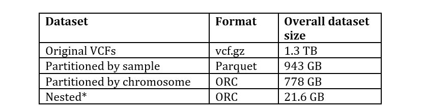
*Contains only selected fields

Amazon Athena has the advantage of being serverless and paying only for queries run. However, as the size of the data in the data lake grows to thousands of whole genomes, some queries could take several minutes to return results. There are some strategies to mitigate this, some of which have been discussed, i.e., using partitioning, nesting, or other techniques to reduce the data amount that must be scanned based on query patterns. However, this does require a significant amount of data engineering to define optimal schemas as the scale of data approaches hundreds of thousands of whole genome data. Users expect interactive queries to return within 10s of seconds, which is not feasible for population level analysis containing 10 billion variants (rows). Particularly, when queries require joins of multiple tables, such as variant data with annotation data, which is a frequent pattern in genomics data, the performance can slow down with large numbers of rows.

Joining separate variant and annotation tables can also slow query response times. One approach is to de-normalize the tables and store the information together. However, annotations are often updated at regular frequencies (e.g., yearly, quarterly, and monthly). To stay relevant and accurate, add an ETL pipeline to update the de-normalized table periodically and document the annotation version.

Amazon Redshift for high performance and scale

In scenarios where the scale of data is very large (> 10,000 whole genomes), and interactive query performance (in the order of 10s of seconds) is important, Amazon Redshift should be used to store the variants and annotation tables. There are several advantages with Amazon Redshift:

1. Compute and storage can be independently scaled on Amazon Redshift with RA3 instance type to achieve the desired performance and scale.
2. Annotation tables can be maintained separately even at large scale. Amazon Redshift supports various distribution styles and can process large table join quickly and complete analysis interactively. The updates to these tables can be managed more easily using insert/merge operations.
3. Since Redshift has many built-in performance tuning enhancements and auto maintenance capabilities, it eliminates the need to perform data engineering operations such as re-partitioning and re-sorting that would be required with Athena as the size of the data increases.

Data can be loaded into Redshift from the S3 data lake using the following:

create table vardata 
distkey(variant_id)
sortkey(chrom, sample_id)
as 
select <frequently accessed columns> from genomics_datalake.variants;

create table anno_data
distkey(variant_id)
sortkey(chrom, clinvar_clnsig)
as 
select <frequently accessed columns> from genomics_datalake.annotations;

With 10,000 samples, there are 10s of billions of variants. Queries that join large tables like this with large annotation tables could take 10s of minutes in Athena, and potentially exceed the default Athena query timeout, in addition to no longer being interactive. The same queries only take a few seconds or minutes in Redshift, due to superior join performance. It is also possible to improve performance by adding nodes to the Redshift cluster to speed up queries.

The architecture using Redshift as the data store is as follows:

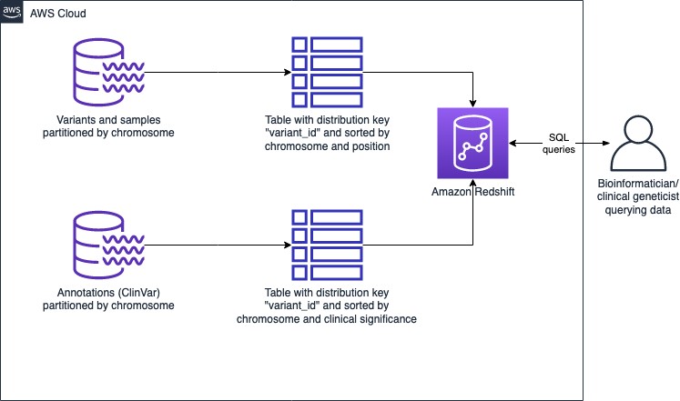
Figure 2: Genomic data store architecture using Amazon Redshift

Example genomics analysis

In both clinical and research scenarios, raw variants are rarely analyzed in isolation without corresponding annotation data. Some common annotation sources include ClinVar for the clinical significance of variants, dbNSFP (in-silico predictions and other annotations all integrated into a single table), gnoMAD (for population allele frequencies), and dbSNP, to name a few. Clinical geneticists and researchers typically use multiple filters on annotations to find the variants or cohort of interest. For example, a clinical geneticist trying to identify causative variants for a specific phenotype in a patient might use filters like genes, regions, HPO phenotype, clinical significance, and population allele frequency from gnoMAD (< 0.01 or < 0.05 indicates rare variants that are more likely implicated in disease). The following is a sample query using annotations from ClinVar and population allele frequencies from gnomAD for the BRCA1 gene:

SELECT * FROM genomics_datalake.var_partby_chrom as v 
           JOIN genomics_datalake.gnomad AS a  
           ON v.variant_id = a.variant_id 
           JOIN genomics_datalake.clinvar as clin
           on a.variant_id = clin.variant_id
           WHERE v.chrom='chr17' AND
           v.pos BETWEEN 43044295 AND 43125364 AND
           cardinality(filter(info_af, x -> x < 0.01)) > 0 
           AND a.info_an > 1 
           AND (clin.clinicalsignificance ='Pathogenic' OR
                clin.clinicalsignificance = 'Likely pathogenic'

For the end user who is a researcher performing analyses at a cohort level, the typical types of queries are used to identify samples that meet a specific criterion. For example, samples that have variants in a specific gene or region, samples that have a pathogenic or likely pathogenic variant in a specific gene, and samples that have rare (minor allele frequency < 0.01) variants in a specific region. The typical mode of operation would be to interactively query using progressively narrower filters to identify a cohort of an appropriate size, and then fetch all of the details about the variants and samples themselves. The following is an example set of queries where a researcher is looking for samples that have Variants Of Uncertain Significance (VUS) variants in the BRCA1 gene, which is present on chromosome 17 between the loci, 43,044,295 and 43,125,364. We will use clinical annotations from ClinVar to do this. To make it easier to join the variants from 1000 Genomes with ClinVar data, we can create a “view” that creates a variant_id field and only includes the fields of interest from the ClinVar summary table. For more on the use of views in Athena, please see here.

create or replace view clinvar as
select concat('chr', chromosome, ':', referenceallelevcf, ':', alternateallelevcf, ':', cast(positionvcf as varchar)) as variant_id
, chromosome as chrom
, positionvcf as pos
, referenceallelevcf as ref
, alternateallelevcf as alt
, genesymbol as genename
, clinicalsignificance as clinvar_clnsig
, numbersubmitters as num_submitters
, reviewstatus as reviewstatus
, split(phenotypeids, ',') as phenotypeids
, split(phenotypelist, ',') as phenotypelist
from "clinvar_summary_variants_dl-awsroda"."variant_summary" where assembly = 'GRCh38'
and referenceallelevcf <> 'na' 
and alternateallelevcf <> 'na'

Then, we can use this “clinvar” view in subsequent queries, such as to further filter the original query by searching for only those samples that have variants of Uncertain Significance (VUS). To increase confidence in the results, we will also look for only those variants that have been labeled VUS by more than one lab.

select count(DISTINCT(sample.id)) from (
  select samples from thousand_genomes.var_nested as v 
  join clinvar a
  on v.variant_id = a.variant_id
  where a.clinvar_clnsig = 'Uncertain significance' 
    and v.chrom='chr17' 
    and v.pos between 43044295 and 43125364
    and a.num_submitters > 1
  ) as f,
unnest(f.samples) as s(sample);

This query returns a result set of 41 samples, which can then be investigated further.

For more example queries and scenarios, we have created a sample notebook here.

Conclusion

In part 1 of this series, we discussed how to transform genomic data to make it optimal to ingest into a data lake and make it query-ready. In this post, we talk about various design and schema choices for the data that impact the performance of queries. We discussed the tradeoffs and considerations between Amazon Athena, which is serverless, and Amazon Redshift, which can offer superior performance at a large scale. We provided examples of some typical patterns of queries on genomic variants, and annotation data and which type of schema might work for each of them.

For more information on Amazon services in Healthcare, life sciences, and genomics, please visit aws.amazon.com/health.

________________________________________________

We’d like to acknowledge the contributions of former colleague Juan Yu – Senior Specialist Solutions Architect, Analytics.