Using R with Amazon Web Services for document analysis

This article is a guest post from David Kretch, Lead Data Scientist at Summit Consulting.

In our previous post, we covered the basics of R and common workload pairings for R on AWS. In this second article in a two-part series, we’ll take a deeper dive on building a document processing application with AWS services. We’ll go over how you can use AWS with R to create a data pipeline for extracting data from PDFs for future processing.

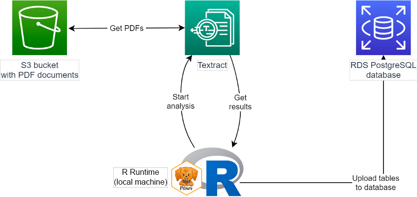
In this example, we’ll start with PDFs stored in Amazon Simple Storage Service (Amazon S3), extract information in the form of text and tables using Amazon Textract, and then upload the data to a PostgreSQL Amazon Relational Database Service (Amazon RDS) database. We’ll access all of these services from our R runtime using the Paws AWS SDK. The diagram below shows how this works.

chart showing flow of getting data from PDFs using R with Amazon Textract and RDS

For researchers, a large amount of valuable data from PDFs and images is difficult to extract for analysis. Examples include SEC Form 10-K annual financial reports, scans of newspaper articles, historical documents, FOIA responses, and so on. Analyzing data from these can be logistically impractical, but now with better machine learning technology, we can start to use these as data sources for research.

In the example in this article, we’re using PDFs of documents containing historical projections of the US economy made by the Federal Reserve, known as the Greenbook projections (or Greenbook Data Sets). These PDFs consist of text with tables and graphs interspersed throughout, adding additional challenges. The Greenbook projections are available from the Philadelphia Federal Reserve.

In this article, we assume you already have an existing S3 bucket with PDFs and an Amazon RDS database. Although you can create these AWS resources from within R, we recommend that you instead use a tool designed for provisioning infrastructure, such as AWS CloudFormation, the AWS Management Console, or Terraform.

We also assume you have already configured local credentials for accessing Amazon Textract. You can achieve this either by importing environment variables and storing them in credential files, or by running R on an EC2 instance or in a container with an attached AWS Identity and Access Management (IAM) role with appropriate permissions. If not, you’ll have to provide credentials explicitly; you can see documentation about doing that in the previous article and with explicit instructions in the Paws documentation.

Extracting text and tables

PDFs are notoriously hard to extract data from. The earliest Greenbook projection PDFs are images of the original report pages made in the 1960s. The more recent ones use the PDF layout language, but even then, there is no underlying structure in a PDF—only characters positioned at points on a page.

To get usable data out of these PDFs, one must use optical character recognition to convert images of text to characters (where needed), then infer sentence, paragraph, and section structure based on where characters fall on a page. The Greenbook projections also contain tables. Here, we need to identify where the tables are, then reconstruct their rows and columns based on the position and spacing of the words or numbers on the page.

To do this we use Amazon Textract, an AWS-managed AI service, to get data from images and PDFs. With the Paws SDK for R, we can get a PDF document’s text using the operation start_document_text_detection and get a document’s tables and forms using the operation start_document_analysis.

These are asynchronous operations, which means that they will initialize text detection and document analysis jobs, returning an identifier for the specific jobs that we can poll to check the completion status. Once the job is finished, we can then retrieve the result with a second operation, get_document_text_detection and get_document_analysis respectively, by passing in the job IDs.

We get the table data for a single document using the following code. We tell Amazon Textract where the document is in our S3 bucket, and it returns us an ID for the document analysis job it will start. In the background, Textract reads in the file and does its analysis. Meanwhile, we can continue to check whether the job is finished, and once it has, get the result.

textract <- paws::textract()

analyze_document <- function(bucket, file) {
  
  # Start analyzing the PDF.
  resp <- textract$start_document_analysis(
    DocumentLocation = list(
      S3Object = list(Bucket = bucket, Name = file)
    ),
    FeatureTypes = "TABLES"
  )
  
  # Check that the analysis is done and get the result.
  count <- 0
  while (count < 30 && (!exists("result") || result$JobStatus == "IN_PROGRESS")) {
    Sys.sleep(1)
    result <- textract$get_document_analysis(
      JobId = resp$JobId
    ) 
    count <- count + 1
  }
  return(result)
}

analysis <- analyze_document("my-bucket", "GS-1966-01-11.pdf")

This is a simplified example; in practice, we would likely start all our document analysis jobs at once, then collect all the results later, as the the jobs can run in parallel. Additionally, analysis results may be too large to be sent all at once, and you may have to get additional parts separately; the full source code listing available at the end of this article does handle this situation.

The result we get back from a Textract document analysis job is divided into blocks. For documents with tables, some blocks are TABLE blocks, the table’s cells are in CELL blocks, and a cell’s contents are in WORD blocks. You can read more about how these work in the Textract Tables documentation.

Now we need to turn the Textract result into a shape we can use more easily. First, let’s look at a table in its original form and how that table is returned to us by Textract. Below is the table from page three of the January 1966 document.
pdf screenshot of Greenbook Projects table, January 1966

And here are three example blocks returned from the Textract analysis:

1. This is the block for this table; you can see below that this is of BlockType TABLE, it is from page 3 (in the Page element), and it has 256 child blocks (the cells) under Relationships.

# List of 13
# $ BlockType      : chr "TABLE"
# $ Confidence     : num 100
# $ Text           : chr(0) 
# $ RowIndex       : int(0) 
# $ ColumnIndex    : int(0) 
# $ RowSpan        : int(0) 
# $ ColumnSpan     : int(0) 
# $ Geometry       :List of 2
# .. <not shown>
# $ Id             : chr "c6841638-d3e0-414b-af12-b94ed34aac8a"
# $ Relationships  :List of 1
# ..$ :List of 2
# .. ..$ Type: chr "CHILD"
# .. ..$ Ids : chr [1:256] "e1866e80-0ef0-4bdd-a6fd-9508bb833c03" ...
# $ EntityTypes    : list()
# $ SelectionStatus: chr(0) 
# $ Page           : int 3

2. This is a block for the cell from row 1, column 2 of the table, as shown by the RowIndex and ColumnIndex elements. This cell has one child block.

# List of 13
# $ BlockType      : chr "CELL"
# $ Confidence     : num 100
# $ Text           : chr(0) 
# $ RowIndex       : int 1
# $ ColumnIndex    : int 2
# $ RowSpan        : int 1
# $ ColumnSpan     : int 1
# $ Geometry       :List of 2
# .. <not shown>
# $ Id             : chr "132b0343-0172-4ddd-bf30-12f133f0f31d"
# $ Relationships  :List of 1
# ..$ :List of 2
# .. ..$ Type: chr "CHILD"
# .. ..$ Ids : chr "5734871f-5a7f-460e-a5f5-dd42bbc57a27"
# ...

3. And finally, a block for the word in the cell above, which contains the text Year.

# List of 13
# $ BlockType      : chr "WORD"
# $ Confidence     : num 99.8
# $ Text           : chr "Year"
# ...

To reconstruct the table, we combine all the cells in the table using each cell’s row and column numbers. The code below does this; it will return a list of all tables in a document, each in matrix form. The code does this by:

iterating across each table’s cells one-by-one
extracting each cell’s contents from their word blocks
inserting the cell contents into the in-memory table’s matrix in the appropriate row and column

get_tables <- function(analysis) {
  tables <- list()
  blocks <- analysis$Blocks
  names(blocks) <- sapply(blocks, function(x) x$Id)

  for (block in blocks) {
    
    if (block$BlockType == "TABLE") {
      cells <- get_children(block, blocks)
      rows <- max(sapply(cells, function(x) x$RowIndex))
      cols <- max(sapply(cells, function(x) x$ColumnIndex))
      table <- matrix(nrow = rows, ncol = cols)
      
      # 1. Go through a table's cells one-by-one
      for (cell in cells) {
        
        # 2. Get the cell's contents
        words <- get_children(cell, blocks)
        text <- paste(sapply(words, function(x) x$Text), collapse = " ")
        
        # 3. Insert the cell contents into the matrix
        row <- cell$RowIndex
        col <- cell$ColumnIndex
        table[row, col] <- text
      }
      tables <- c(tables, list(table))
    }
  }
  return(tables)
} 

tables <- get_tables(analysis)

Note that the get_children function above gets a block’s child blocks; it is omitted here for brevity, but appears in the source code listing available at the end of this article.

This code produces a matrix that looks like this, which is pretty good:
Table showing Textract results converted to an R matrix

To run this same process on all our PDFs, we just need to get a list of PDFs from S3, which we can get using the S3 list_objects operation. Then we can loop over all the available PDFs and have Textract get their text and tables via multiple parallel processing jobs.

Uploading data to the database

Now that we have the tables, we are going to upload them to our PostgreSQL database to enable further downstream analysis at a later point.

A suitably configured PostgreSQL server running on RDS supports authentication via IAM, avoiding the need to store passwords. If we are using an IAM user or role with the appropriate permissions, we can then connect to our PostgreSQL database from R using an IAM authentication token. The Paws package supports this feature as well; functionality that was developed using the support of the AWS Open Source program.
We connect to our database using the token generated by build_auth_token from the Paws package.

# Connect to the database using an IAM authentication token.
rds <- paws::rds()
token <- rds$build_auth_token("myhost:5432", "us-east-1", "david")
con <- DBI::dbConnect(
    RPostgres::Postgres(),
    host = "myhost", port = 5432, dbname = "mydb",
    user = "david", password = token
)

With that connection, we upload our results to a table in the database. Because the tables that we get from a document don’t necessarily all have the same shape, we upload them as JSON data. One of the features of PostgreSQL is that it natively allows us to store data of any shape in JSON columns.

# Create rows for each table to insert into the database.
database_rows <- data.frame(
  document = "GS-1966-01-11.pdf", 
  table_num = 1:length(tables),
  data = sapply(tables, jsonlite::toJSON)
)

# Store the tables in the database.
DBI::dbAppendTable(con, name = "tables", value = database_rows)

Now that it’s in the database, we have easy access to it for any future analysis.

Next steps

In this implementation, documents are processed one at a time (and in order) because R is single-threaded by default. In a more complex implementation, we could use the parallel or futures packages to process these documents in parallel, or without waiting for each to finish. Because of the added complexity, we avoided showing that in this article. For those looking to add automation, one could set S3 file uploads as an event trigger for invoking a downstream compute service (Lambda, ECS) that could execute the code referenced here.

Source code

# Using R with Amazon Web Services for document analysis
# https://aws.amazon.com/blogs/opensource/using-r-with-amazon-web-services-for-document-analysis/

# This R program shows how you can use AWS with R to create a data pipeline for
# extracting data from PDFs for future processing, using Textract, S3,
# Relational Database Service (RDS).

# The PDF document is from the Greenbook projections, a set of economic 
# projections made by the Federal Reserve from 1966 to the present.  They are
# available as a collection of PDFs from the Philadelphia Federal Reserve at:
# https://www.philadelphiafed.org/research-and-data/real-time-center/greenbook-data/pdf-data-set

# This R program expects that you have:
#   - An S3 bucket with PDFs
#   - An RDS PostgreSQL database with IAM authentication
#   - A user, instance, or container with IAM permissions to access Textract
#     and your RDS database
#   - R, and the packages paws, DBI, and RPostgres

#-------------------------------------------------------------------------------

# The location of the first Greenbook Projections PDF document in S3.
bucket <- "my-bucket"
file <- "GS-1966-01-11.pdf"

textract <- paws::textract()

#-------------------------------------------------------------------------------
#-------------------------------------------------------------------------------
#-------------------------------------------------------------------------------

# Get a PDF document's tables using Amazon Textract.
# --------------------------------------------------

analyze_document <- function(bucket, file) {
  
  # Start analyzing the PDF.
  resp <- textract$start_document_analysis(
    DocumentLocation = list(
      S3Object = list(Bucket = bucket, Name = file)
    ),
    FeatureTypes = "TABLES"
  )
  
  # Check that the analysis is done and get the result.
  count <- 0
  while (count < 30 && (!exists("result") || result$JobStatus == "IN_PROGRESS")) {
    Sys.sleep(1)
    result <- textract$get_document_analysis(
      JobId = resp$JobId
    )
    # If the result has multiple parts, get the remaining parts.
    next_token <- result$NextToken
    while (length(next_token) > 0) {
      next_result <- textract$get_document_analysis(
        JobId = resp$JobId,
        NextToken = next_token
      )
      result$Blocks <- c(result$Blocks, next_result$Blocks)
      next_token <- next_result$NextToken
    }
    count <- count + 1
  }
  
  return(result)
}

analysis <- analyze_document(bucket, file)

#-------------------------------------------------------------------------------
#-------------------------------------------------------------------------------
#-------------------------------------------------------------------------------

# Turn the Textract analysis result into matrices.
# ------------------------------------------------

# Get all children for a given block.
get_children <- function(block, data) {
  if (length(block$Relationships) == 0) {
    return(list())
  }
  idx <- which(sapply(block$Relationships, function(x) x$Type) == "CHILD")
  if (!idx) {
    return(list())
  }
  child_ids <- block$Relationships[[idx]]$Ids
  result <- data[child_ids]
  return(result)
}

# Get all tables for a given document analysis returned by `analyze_document`.
get_tables <- function(analysis) {
  blocks <- analysis$Blocks
  names(blocks) <- sapply(blocks, function(x) x$Id)
  tables <- list()
  for (block in blocks) {
    
    if (block$BlockType == "TABLE") {
      cells <- get_children(block, blocks)
      rows <- max(sapply(cells, function(x) x$RowIndex))
      cols <- max(sapply(cells, function(x) x$ColumnIndex))
      table <- matrix(nrow = rows, ncol = cols)
      
      # 1. Go through a table's cells one-by-one
      for (cell in cells) {
        
        # 2. Get the cell's contents
        words <- get_children(cell, blocks)
        text <- paste(sapply(words, function(x) x$Text), collapse = " ")
        
        # 3. Insert the cell contents into the matrix
        row <- cell$RowIndex
        col <- cell$ColumnIndex
        table[row, col] <- text
      }
      tables <- c(tables, list(table))
    }
  }
  return(tables)
}

tables <- get_tables(analysis)

#-------------------------------------------------------------------------------
#-------------------------------------------------------------------------------
#-------------------------------------------------------------------------------

# Upload our results to our database.
# -----------------------------------

# Connect to the database using an IAM authentication token.
rds <- paws::rds()
token <- rds$build_auth_token("myhost:5432", "us-east-1", "david")
con <- DBI::dbConnect(
  RPostgres::Postgres(),
  host = "myhost", port = 5432, dbname = "mydb",
  user = "david", password = token
)

# Create rows for each table to insert into the database.
database_rows <- data.frame(
  document = "GS-1966-01-11.pdf", 
  table_num = 1:length(tables),
  data = sapply(tables, jsonlite::toJSON)
)

# Store the tables in the database.
DBI::dbAppendTable(con, name = "tables", value = database_rows)

David Kretch

David Kretch is Lead Data Scientist at Summit Consulting, where he builds data analysis systems and software for the firm’s clients among the federal government and private industry. He, alongside Adam Banker, is also coauthor to Paws, an AWS SDK for the R programming language. Adam Banker is a full-stack developer at Smylen and also contributed to this article.

The content and opinions in this post are those of the third-party author and AWS is not responsible for the content or accuracy of this post.

Feature image via Pixabay.