Analyzing petabytes of trade and quote data with Amazon FinSpace

We recently announced Amazon FinSpace, a fully-managed data management and analytics service that makes it easy to store, catalog, and prepare financial industry data at scale, reducing the time it takes for financial services industry (FSI) customers to find and access all types of financial data for analysis from months to minutes. Financial services organizations analyze data from internal data stores like portfolio, actuarial, and risk management systems, as well as petabytes of data from third-party data feeds, such as historical securities prices from stock exchanges. It can take months to find the right data, get permissions to access the data in a compliant way, and prepare it for analysis.

FinSpace removes the heavy lifting of building and maintaining a data management solution for financial services. With FinSpace, you can collect, manage, and catalog data by your relevant business concepts, such as asset class, risk classification, or geographic region, which makes it easy to discover and share across your organization. FinSpace includes a library of over 100 functions, such as time bars and realized volatility, to prepare data for analysis. You can also integrate functions from your own libraries and notebooks for your analysis. FinSpace supports your organization’s compliance requirements by ensuring data access controls are enforced and maintaining data access audit logs.

This post introduces you to the Amazon FinSpace time series framework, discusses its benefits, and demonstrates how you can use it.

Time series analysis is performed to extract insights from historical event data to guide business decisions. This kind of analysis is widely used in the financial services industry. You might integrate a number of tools for specialized software solutions, compute capacity, data storage, and databases to carry out time series analysis. The data used in the time series analysis is typically large in size and contains hundreds of billions of events. For example, the size of historical US Equities TAQ data is approximately 5 TB a year and contains more than 250 billion data events, having increased 300% over the past 5 years. Analyzing such large time series datasets is a challenge because of scaling limits of specialized software solutions, compute, and storage in your on-premise environments. These challenges limit your ability to respond to scale with data volume and the need for more analytics. For example, in volatile markets when data volumes grow rapidly and business needs require more analytics than usual, a scale-constrained solution results in a financial disadvantage.

Amazon FinSpace provides all the functionality required to perform time series analysis at scale. Time series data can be ingested into FinSpace from sources such as vendor data feeds, on-premises data centers, and enterprise data lakes. With the bi-temporal data management engine of FinSpace, you can track data versions, corrections, and create point-in-time views. You don’t need specialized hardware or software; you run analysis from Jupyter notebooks integrated with dynamically scalable Spark compute clusters. The framework is delivered as a library with over 100 FinSpace time series functions, and you can bring your own functions or use open-source libraries that can be scaled on Spark. There are no constraints on storage or compute; both scale dynamically based on your data and computational needs. To begin time series analysis, add a dataset to FinSpace or choose an existing dataset from the FinSpace catalog, open it in a FinSpace notebook with a managed Spark cluster, and start using the framework.

What is the Amazon FinSpace time series framework?

The FinSpace time series framework defines a set of stages to transform data from raw time series data events to the computation of finance-specific analytics like technical indicators. The FinSpace time series functions are used in different stages. Each stage accepts inputs from the previous stage and acts as an input to the next stage. You can slot your own functions at any stage. The path through the stages of analysis can change depending on the input time series data events being dense or sparse. An example of dense data (high-resolution data) is historical US Options Price Reporting Authority (OPRA) data, which contains tens of billions of daily events. An example of sparse data is treasury data where yields on maturities that lie between the on-the-run treasuries aren’t available and are generated by interpolation.

The following diagram illustrates the stages of the Amazon FinSpace time series framework.

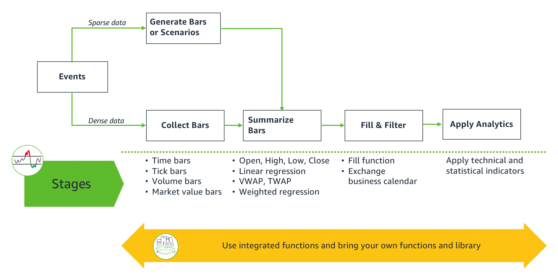
Analysis begins with raw time series events data that is input to the following stages in the framework:

• Collect Bars – This stage is applicable to processing dense event data. The objective of this stage is to collect the series of events that arrive at an irregular frequency into uniform intervals called bars. You can perform collection with your functions or use the FinSpace functions to calculate bars, such as the following:
  • Time bars – Collect events at fixed time intervals. For example, for a given day of trading prices for AMZN (Amazon) from the US Equities NYSE TAQ dataset, FinSpace analytical functions can be used to collect 1-minute time bars, where each bar is the collection of trading price events that occurred for each interval of the day.
  • Tick bars – Collect events at each predefined number of events (for example, collect events at one bar every 100 events).
  • Volume bars – Collect events after a predefined number of security units have been exchanged.
  • Market value bars – Collect events after a predefined market value is exchanged.
• Generate Bars or Scenarios – This stage is applicable to sparse data where input events may not be enough to collect into bars. The objective of this stage is to generate bars that can serve as input to next stage. You can bring your own functions to generate bars. For example, a fixed income analyst can generate bars for prices on a bond that had no trades during a time interval by interpolating from available prices for the same bond during another time interval. You may also generate scenarios on existing datasets to assess the impact of a trading strategy, such as shifting the trading price by a percentage and generating a new time series dataset for a what-if analysis. This technique is used often in options analysis where the spot price is shifted by a percentage to create new datasets from an existing dataset.
• Summarize Bars – The objective of this stage is to take collected data in bars from the previous stages and summarize them. For example, an asset manager can use US Equities NYSE TAQ event data to summarize those events into 1-minute bars. You can derive Volume Weighted Average Price (VWAP) summaries, a trading benchmark used to calculate the average price a security has traded at throughout the day, based on both volume and price. You can perform your own summaries or use the analytical functions provided for this stage to calculate weighted linear regression, total volume, and OHLC (open, high, low, close) prices.
• Fill and Filter – The data produced in the previous stage could have missing bars where no data was collected or contain data that you don’t want to use in the next stage. The objective of this stage is to prepare a dataset with evenly spaced intervals and filter out any data outside the desired time window. For example, if no activity occurred in a period of time, no data is summarized. This means that missing (empty) summary bars must be added to the data to account for periods in which no data was collected. This filling can be a simple insertion of NaN values (Not a Number) or could take into account what the empty bar represents and use an appropriate value. The framework provides a default fill function. The resulting dataset is filtered out based on a trading holiday and exchange hours calendar. FinSpace provides the NYSE business calendar, or you can use your own. The prepared dataset of features is now ready for the next stage.
• Apply Analytics – At this stage, a prepared dataset of features is ready for application of technical and statistical indicators. You can bring your own indicator functions or choose one of the FinSpace functions for this stage, including moving average, converge/diverge (MACD), Ichimoku, relative strength indicator (RSI), and commodity channel index (CCI). The output of this stage can be an input to your analytical functions, or a summary statistic that is a response to a business problem defined at the beginning of the analysis.

Getting started with the time series framework

Our use case shows how a dataset with dense raw time series events is transformed through the stages of the FinSpace time series framework. The input dataset used is US Equities Trades & Quotes (TAQ) data with a 3-month history (2019-10-01 to 2019-12-01) for Amazon traded under symbol AMZN. The code and the output in the FinSpace Jupyter notebook demonstrates the stages that process the raw events and calculate Bollinger Bands. Although the analysis runs on the full dataset, for the purposes of this post, the screenshots only show a handful of events as of 2019-10-01 at market open at 9:30 AM to follow the output easily.

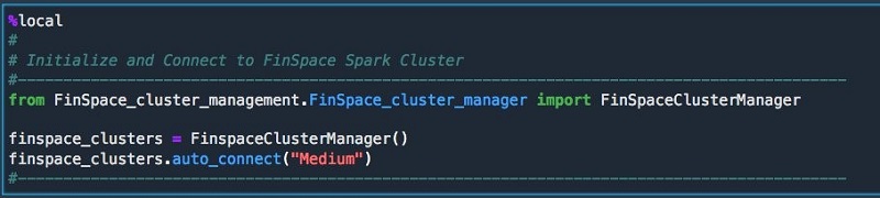
You begin by starting and connecting to the Spark cluster. If no running cluster is found, a cluster is created.

Next, you initialize FinSpace dataset and data view identifiers. You can get the dataset ID and data view ID from the FinSpace Dataset page.

Read the data view into a Spark DataFrame.

The data view now loaded into the DataFrame contains raw data events. The DataFrame is filtered on ticker, eventtype, datetime, price, quantity, exchange, and conditions fields.

In the Collect Bars stage, the FinSpace create_time_bars function collects raw data events into 1-minute time bars.

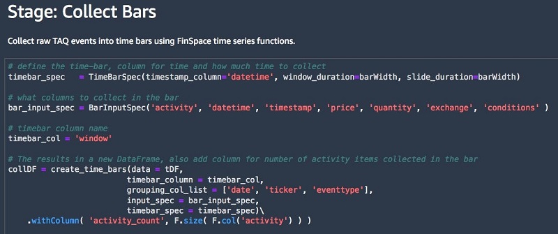
The window represents the 1-minute time interval for the bar. The activity_count shows the number of events collected in each bar. The data events collected inside the bar are not shown.

In the Summarize Bars stage, the FinSpace summarize functions are applied to calculate 1-minute summaries of events collected in bars. Summaries are created for two-point standard deviation, Volume Weighted Average Price, and open(first), high, low, and close(last) prices (OHLC).

The activity count shows the number of events summarized in a single summary bar.

In the Fill and Filter stage, the resulting dataset is filtered according to an exchange trading calendar.

The schema is simplified to prepare a dataset of features.

In the Apply Analytics phase, the FinSpace Bollinger Bands function is applied on the features dataset. The tenor window to perform the calculation is 15, which means that the calculation is applied when 15 data events are available.

Because each event corresponds to a 1-minute summary bar in the features dataset, the resulting dataset starts from timestamp 09:45 (see end column).

You can plot the output into a chart using matplotlib. The following chart shows the Bollinger Bands for the entire 3-month history for AMZN.

The example dataset is part of the sample data bundle with Amazon FinSpace. You can download the notebook. The dataset used in the example is from Algoseek.com.

Conclusion

In this post, we introduced the Amazon FinSpace time series framework, which enables you to analyze large time series datasets and scale as the size of the datasets grows with ever-increasing market activity. The FinSpace Time series framework is available to use now. For more information, visit https://docs.aws.amazon.com/finspace.

About the Authors

Vincent Saulys is a Principal Solution Architect at AWS working on FinSpace. Vincent has over 25 years of experience solving some of the world’s most difficult technical problems in the financial services industry. Launcher and leader of many mission-critical breakthroughs in data science and technology on behalf of Goldman Sachs, FINRA, and AWS.

Steve Yalovitser is a life long learner, and Principal Engineer at AWS, working on FinSpace. Steve has spent over 30 years building systems in capital markets, starting on PDP 11s with MODULA-2. He is passionate about customer problems in finance, and is constantly looking for ways to innovate on their behalf. His innovations in addition to FinSpace include large scale distributed systems for historical analysis, CVA and CCAR for Wells Fargo, and BAML.

Piyush Khandelwal is a Product Manager at AWS, working on FinSpace. Piyush has over 10 years of experience helping customers deploy real-time market data solutions in capital markets.