AWS Open Source Blog
Building the Geomap plugin for Grafana 8.1
In this post, AWS software development intern engineers Bryan Uribe and Eunice Kim talk about their experience with developing the new panel plugin, Geomap, for Grafana. They share goals for the project, key design details, and lessons learned through working on one of the most popular open source projects.
Introducing Grafana and the Geomap plugin
Grafana is a popular open source monitoring platform that allows you to query and visualize metrics from various data sources. With Grafana, you can create complex monitoring dashboards using interactive query builders and personalize the Grafana experience by using of either core or external plugins. A core plugin is included with Grafana, whereas an external plugin must be manually installed.
Geomap is a new core plugin introduced in Grafana 8.1, allowing you to visualize geospatial data. You can customize the world map, configure various overlays, and refine map settings to focus on the important location-based characteristics of data.
The focus of our internship was to design and build the Geomap plugin and contribute the plugin to the open source Grafana project. We worked closely with Ryan McKinley from Grafana Labs to collaborate on the design and development of the new plugin.
Geomap plugin evaluation and design
To understand the Grafana plugin landscape better, we researched existing Worldmap plugins that we could use for our development process. We found an existing Worldmap plugin available for open source Grafana users and investigated whether it could work on top of the existing code. This plugin, however, has not been recently maintained and is limited in the types of base maps and overlays it can support.
We also determined that, because of its non-modular design, the existing plugin would require extensive work before new enhancements could be added. Specifically, functionality for user interactions, loading the base map, generating the circle overlay, and the creation of legends and tooltips are all tightly integrated in the main Worldmap component. This design prevents us from being able to extend the plugin easily to include additional features, such as a configurable tile server, because new enhancements must conform to a standardized component initialization flow.
Moreover, the Worldmap plugin is written in AngularJS, and Grafana has been migrating all of its plugins from AngularJS to React. Grafana is actively encouraging developers to write new plugins using React for the following reasons:
- React/Redux will naturally introduce an architecture that separates the UI from the state. Previously, component, services, and utilities were tied together, which meant that any change in a plugin mutated all the pieces.
- Grafana provides React plugin APIs that can be used to develop plugins. Commonly used UIs and functionalities can be standardized throughout various Grafana plugins.

Figure 1: Geomap plugin project overview.
With increasing use cases and demand for mapping visualizations, the Grafana community has been requesting more features than currently exist in the Worldmap plugin. Thus, we ultimately decided to build a new React Geomap plugin that addresses the concerns of scalability in the Worldmap plugin. A visual overview is shown in Figure 1.
Our key design decisions for this plugin include:
- Building the new plugin in React
- Creating an easily scalable architecture
- Adding a flexible base map configuration
These design decisions were intended to ensure that future development can be integrated easily into the plugin. In particular, this flexibility was provided by removing the tight integration of the Worldmap components.
In the new Geomap plugin, the base maps and data-driven layers are instantiated using a layer handler. This layer handler is responsible for initializing the various layers and allows each layer to carry its own functionality. Each layer is responsible for supplying an initialization function, an optional update function, and an optional legend.
The separation of components through the layer handler means that each data-driven layer can hold its own data formatting processes. Different overlays can customize their data-mapping logic, and the Geomap can interchange various data-driven overlays without adhering to a standardized data flow. In the new design, each layer will be able to determine how to process user data through its own update function (Figure 2).

Figure 2: Geomap plugin architecture.
Configuration
Base layer server configuration
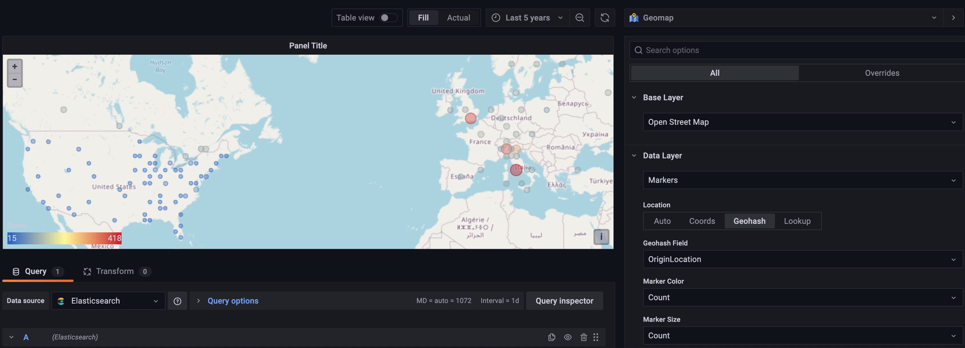
The base layer is the starting point for all Geomap panels. The Geomap layer handler loads a static base layer from a selected tile server to the Grafana panel. You can choose from several base layer options, such as CartoDB, OpenStreetMap, and ArcGIS (Figure 3).

Figure 3: Base layer options available in the Geomap plugin.
In addition to various predefined base layers, we built an extra level of configurability for provisioning of the default base layer. Two new environment variables are now included in the .ini configuration file to configure the default base layer and deactivate the other preconfigured base layer options.
- The JSON configuration option
default_baselayer_configdefines the default base map. Currently there are four base map options to choose from:carto,esri-xyz,osm-standard, andxyz. Thexyzoption allows pointing to a custom tile server URL. - The Boolean configuration option
enable_custom_baselayersenables the predefined base maps. This option is set to true by default, but it can be switched if a service requires loading only one specific base map.
An example use case is when offline access for the base map is required. Although Grafana itself does not require an internet connection, some map panels need internet access to reach a base layer endpoint. Allowing you to configure your own base layer lets you also configure one that is compatible offline (Figure 4).

Figure 4: Base layer configured through provisioning.
Data layer (overlays)
The Geomap panel supports displaying a map overlaid with markers (such as circles) or a heatmap. Each data layer has the option to format user data and tie its location-based metrics into the style of the overlay. Further details can be found in the data-mapping section of this article.
Markers layer
The markers layer enables the visualization of data points with different marker shapes, such as circle, square, triangle, star, cross, and X (Figure 5).
- Marker color configures the color of the marker. The default
Fixed colorkeeps all points a single color. An alternate option is to have multiple colors depending on the data point values and the threshold set at theThresholdssection. - Marker size configures the size of the marker. The default
Fixed valuemakes all marker sizes the same regardless of the data point metric. There also is an option to scale the circles to the corresponding data point metric.MinandMaxmarker size scales the marker size to the specified range. - Marker shape provides the flexibility to change the marker style. Possible choices for marker shapes are: circle, square, triangle, star, cross, and X.
- Fill opacity configures the transparency of each marker.
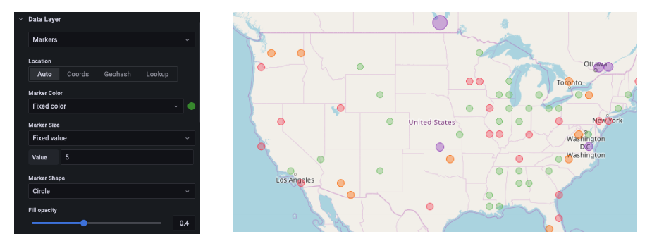
Figure 5: Data layer UI using Markers overlays.
Heatmap layer
The heatmap layer clusters data points to visualize locations with different densities. As with the markers layer, you are prompted to configure various options to customize the visualization (Figure 6).
- Weight values configures the intensity of the heatmap clusters.
Fixed valuekeeps a constant weight value throughout all the data points. This value should be in the range of 0~1. There is an alternate option to scale the weight values automatically depending on the data values. - Radius configures the size of the heatmap clusters.
- Blur configures the amount of blur on each cluster.
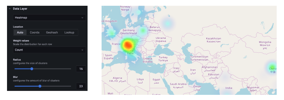
Figure 6: Data layer UI using heatmap overlays.
We use OpenLayers to implement the overlays shown in Figure 6. OpenLayers is an open source JavaScript API for building dynamic map applications. It includes components such as Map, Layer, and Source to render and visualize the map with various overlays.
Map is a core component in OpenLayers and is the starting point for all mapping applications, as it loads in a base map and allows multiple layers to be added on top. Each layer includes a source, which holds information on how to load the layer content. For markers, the source reads data and provides the layer with a set of features to visualize. Each feature includes a geometry property that can be styled to create the desired overlays (Figure 7).

Data mapping
An integral part of the visualization process involves mapping user data to geographical locations. In the Geomap plugin, this process is separated into two steps: finding data fields in user data and creating Geomap points.
This approach provides a more modular and scalable design, as overlays can reuse data-mapping functionality but avoid a tight integration with a specific data-mapping flow. For example, different overlays can reuse data-mapping logic for creating points, but instantiate different styles, such as markers or heatmaps.
Data can come from one of a variety of data sources, such as Elasticsearch, Prometheus, InfluxDB, and so on. The only requirement is that the data source must include location data. This location data must be formatted into one of the following location types: coordinates, geohash, or lookup.
- Coordinates: Longitude and latitude information.
- Geohash: An encoding of coordinates into an alphanumeric string.
- Lookup: A location name that must be matched to a geographical point.
These location options allow the plugin to work with some of the most common databases and provide a flexible data-mapping experience. In the panel UI, you will be prompted to select the location type of the data query. The following four location types are available:
- Coords specifies that the query holds coordinate data. Select the data fields for latitude and longitude from the database query, and the data mapping iterates through those fields to create points. Here, the latitude and longitude are directly used in the creation of points:
- Geohash specifies that the query holds geohash data. Select the data field for geohash from the database query and the data mapping iterates through those fields to create points. Here, the geohash is decoded into latitude and longitude for the creation of points:
- Lookup specifies that the query holds location name data that must be mapped to a value. Select the lookup field from the database query along with the type of gazetteer. The gazetteer is the dictionary that will be used to map queried data to a geographical point. To create a point, the location value is mapped to latitude and longitude using the gazetteer:
- Auto is an automatic data handler that will automatically search for location data. You can select this data option when a query contains one of the following names for data fields. If the data handler finds fields for any of the location options, it will try to use that field to instantiate Geomap points:
- geohash: “geohash”
- latitude: “latitude”, “lat”
- longitude: “longitude”, “lng”, “lon”
- lookup: “lookup”
Data hover (tooltips)
In addition to data layers, tooltips provide an alternative method for displaying user data. Tooltips are essential to the visualization process, because they help us understand metrics that would otherwise be difficult to discern through the overlays themselves. When we hover or pause over a data feature, a tooltip becomes visible, displaying specific information that the feature represents.
For example, the tooltip shown in Figure 8 provides detailed information on the feature’s Count, which is directly correlated to the size and color of the circle marker. This metric would be difficult to distinguish based solely on the size and color of the circle markers.

Figure 8: Tooltip visualization.
Specifically, tooltips are created by instantiating a pointer event handler on the Geomap panel, and listening for when the pointer pauses over a feature. If the pointer pauses over a feature, the properties (defined by user data) of the feature are pulled and sent to the Geomap panel, where a tooltip is generated:
Developing the Geomap plugin
For this project, we built a Grafana plugin to allow you to visualize geographic data. Geomap is a panel plugin, which is one of the four key types of plugins that Grafana implements:
- Data source: Enables communication with databases.
- Backend: Builds alerts for data sources and holds functionality for query caching.
- Panel: Creates custom ways of visualizing data on the front end.
- App: Allows you to create custom styles of monitoring.
Panel plugins are purely front end and are written in TypeScript. In developing the Geomap plugin, we also had to conform to Grafana coding styles, including adhering to code organization protocols, naming conventions, and practices for implementing React components.
Moreover, the development process for creating a core Grafana plugin is different from creating an external plugin. In particular, our development was done through the main Grafana repository and required setting up a Grafana development environment. This process consisted of downloading the source code for Grafana and building the project as described in the guide for developers. The final step was to configure the custom.ini file to put the Grafana application into development mode:
Testing plan
For the Geomap plugin, both unit tests and integration tests were carried out to ensure that all functionalities were working as intended. Specifically, we tested that the panel was created error-free, that the various overlays were instantiated properly, and that the data formatting logic worked correctly.
- Unit tests: The different components of the plugin must have their expected functionalities covered by unit tests. Unit tests follow the conventions and use the frameworks included in the existing Grafana test suite for other panel plugins. Here we used jest, a front-end testing framework, to test the data formatting logic in the front end. The front-end tests can be run using Yarn:
- Integration tests: Grafana’s test suite does not contain automated integration tests for plugins; however, manual verification of the plugin is done with a Grafana build. Each UI component was tested to ensure desired functionalities.
Getting ready to use the Geomap plugin
Let’s look at an example of how to use the Geomap plugin. In this example, we demonstrate how to build a Geomap visualization and use the Markers layer to visualize our sample data query. Although parts of this example will be specific to our data, layer options and configuring thresholds are necessary for any visualization. In particular, we will walk through our sample data, configure the data layer, and set thresholds.
Grafana setup
Geomap is a core plugin in Grafana and is included in Grafana 8.1+. To use the plugin, select Geomap from the available list of visualizations (Figure 9).

Figure 9: Geomap in the available list of visualizations.
Data query
The following table represents our sample data query with a metric and location field. Here, the information displays the number of errors at a location of the same row. Note, that our location data is represented as a geohash.
| Errors | State | |
| 1 | 24 | bdg |
| 2 | 41 | 9q6 |
| 3 | 48 | 9wv |
| 4 | 12 | drt |
Data layer
Under the data layer, select the Markers overlay (Figure 9). You will be prompted to select the location type of your data. Our data query holds geohash data, so you will select the geohash option. Moreover, you must provide the data field that holds the location data, which is State.
At this point, you can select various options to adjust the style of the Markers. Here, you will select the data’s metric field, Errors, to configure the size and colors of the markers. In this demo, the rest of the options are left as default (Figure 10).

Figure 10: Example settings of markers overlay demo.
Thresholds
Thresholds allow custom colors for the markers. These quantities will vary for each dataset and will depend on the scale of the metric used. For our sample data, meaningful thresholds relate to the following: error count below 20 is green, above 20 but below 40 is yellow, and any count of errors above 40 is red (Figure 11).

Figure 11: Example thresholds of markers overlay demo.
Result
Finally, the Geomap panel should look like the visualization shown in Figure 12.
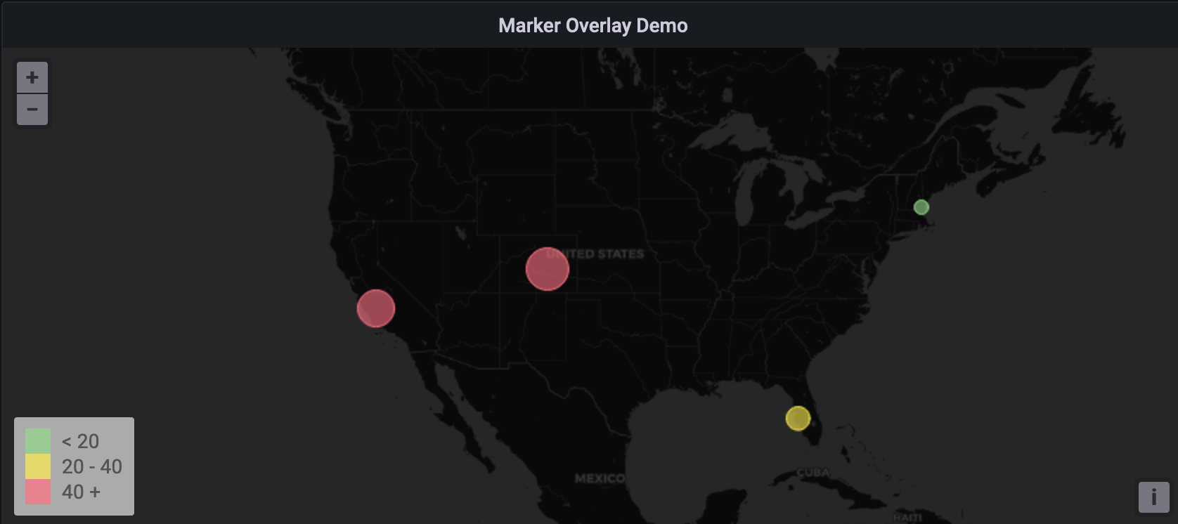
Figure 12: Final visualization.
Conclusion
We were able to build a Geomap plugin for the open source Grafana project in collaboration with Grafana Labs. Our contributions in the form of pull requests (PRs) include changes in the base layer configuration, data layers, data formatting, and tooltips.
Following is the list of PRs we have contributed upstream:
- Implement Circle Overlays
- Implement Heatmap Overlays
- Implement Base Layer Server Configuration
- Implement Default Base Layer
- Implement Geomap Tooltip
- Implement Lookup Mapping
- Test Dataframe To Points
- Update Gazetteer Information
- Document the Geomap Panel Plugin
We are grateful for the feedback and support we received from our technical mentors—Alolita Sharma, Helen Lin, Robbie Rolin, and Ryan McKinley (Grafana Labs)—with whom we worked closely throughout the project. During our internships, we learned a tremendous amount about the open source community and developing open source-approved code. Moreover, we gained experience in writing high-quality TypeScript code, and how to communicate effectively and collaborate with different engineers around the world. We look forward to the widespread use of the Geomap plugin and are excited to see our contributions make a positive change on the user experience of the plugin. As of the publication of this blog post, Grafana 8.1 is already out, and it includes our Geomap plugin. Check out the release announcement and give the Geomap plugin a try! We look forward to hearing any feedback you may have or bugs you find when making your visualizations.

Bryan Uribe
Bryan Uribe is a fourth-year student studying mathematics and computer science at Harvey Mudd College. He is an SDE intern at AWS and is interested in observability and machine learning.

Eunice Kim
Eunice Kim is a fourth-year electrical engineering student at the University of British Columbia. She is an SDE intern at AWS interested in observability and open source projects.