Advanced analytics with table calculations in Amazon QuickSight

Amazon QuickSight recently launched table calculations, which enable you to perform complex calculations on your data to derive meaningful insights. In this blog post, we go through examples of applying these calculations to a sample sales data set so that you can start using these for your own needs.

You can find the sample data set used here.

What are table calculations?

By using a table calculation in Amazon QuickSight, you can derive metrics such as period-over-period trends. You can also create calculations within a specified window to compute metrics within that window, or benchmark against a fixed window calculation. Also, you can perform all these tasks at custom levels of detail. For example, you can compute year-over-year increase in sales within  industries, or the percentage contribution of a particular industry within a state. You can also compute cumulative month-over-month sales within a year, how an industry ranks in sales within a state, and more.

You can compute these metrics using a combination of functions. These functions include runningSum, percentOfTotal, and percentDifference, plus a handful of base partition functions. The base partition functions that you can use for this case include sum, avg, count, distinct_count, rank, and denseRank. They also include minOver and maxOver, which can calculate minimum and maximum over partitions.

Partition functions

Before you apply these calculations, look at the following brief introduction to partition functions. Partitions enable you to specify the dimension that is the window within which a calculation is contained. That is, a partition helps define the window within which a calculation is performed.

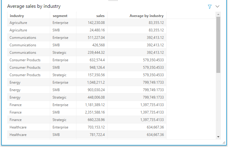
As an example, let’s calculate the average sales within each industry across segments. We start by adding industry, segment, and sales to the visual. Adding a regular calculated field avg(sales) to the table gives the average of each segment within the industry, but not the average across each industry. To achieve this, create a calculated field using the avgOver calculation.

avgOver(aggregated measure, [partition by attribute, ...])

The aggregated measure here refers to the calculation to perform on the measure when it’s grouped by the dimensions in the visual. This calculation occurs before an average is applied within each industry partition.

Average by industry = avgOver(sum(sales), [industry])

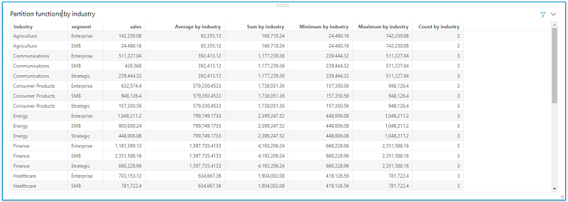
Similarly, you can calculate the sum of sales, minimum and maximum of sales, and count of segments within each industry by using the sumOver, minOver, maxOver, and countOver functions, respectively.

Benchmark vs. actual sales

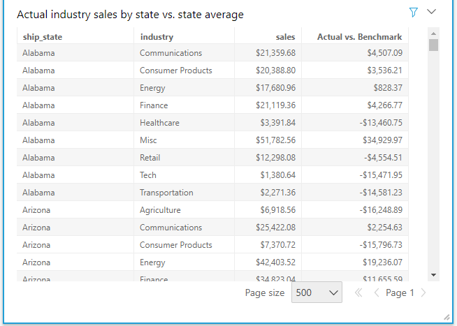
Let’s take another use case and see how each industry within a state performs when benchmarked against the average sales in the state.

To achieve this, add state, industry, and sales to a table visual and sort by the state. To calculate the benchmark, create a calculated field with the avgOver function partitioned by the State dimension.

avgOver(aggregated measure, [partition by attribute, ...])

State average = avgOver(sum(Sales), [ship_state])

Given that we added state, industry, and sales to the table, sum(sales) calculates the total sales of an industry within a state. To determine the variance of this value from the benchmark, simply create another calculated field.

Actual vs. benchmark = sum(sales) – State average

As with the calculations preceding, you can derive the percentage of sales within an industry compared to the total sales within the state by using percentOfTotal calculations.

Running Sum, Difference, and Percent Difference

We can illustrate several more functions with use cases, following.

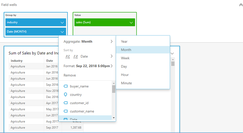
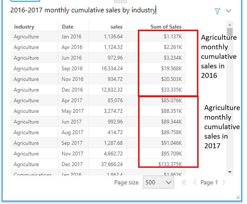
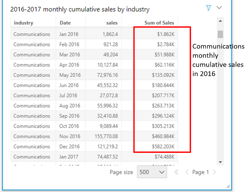
Use case 1: As a sales analyst, I want to create a report that shows cumulative sales by month within each industry from the beginning till the end of each calendar year.

To derive the cumulative monthly sales by industry, I need industry, date, and sales represented in a table chart. After adding the date field, I change the aggregation to month (as shown following).

I add a new calculated field to the analysis using the runningSum function. The runningSum function has the following syntax.

runningSum(aggregated measure, [sort attribute ASC/DESC, ...], [partition by attribute, ...]

The aggregated measure here refers to the aggregation that we want when grouping by the dimensions included in the visual. The sort attribute refers to the attribute that we need sorted before we perform the running sum. As mentioned preceding, partitioning by attribute specifies the dimensions where the running sum is contained within each value of the dimension.

In this use case, the aggregate measure that we want to measure is sum(sales), sorted by date and partitioned by industry and year. Plugging in these attributes, we arrive at the formula following.

runningSum(sum(sales),[Date ASC],[industry, truncDate("YYYY",Date)])

The square brackets within the sort fields and partition lists are mandatory. We then add this calculated field to the visual and sort the order of the industry. Without the partition on year, runningSum calculates the cumulative sum across all months starting from 2016 through the end of 2017.

You can also represent cumulative monthly sales by using line charts and other chart types. In a line chart, the slope of the lines shows the rate at which the industry is growing in a year. For example, the growth of the tech industry seems slow in 2016 but picked up rapidly in 2017.

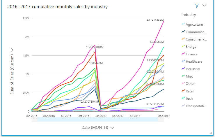
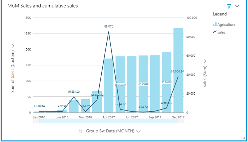
You can also represent the total sales and cumulative sales in a combo chart and filter by the industry.

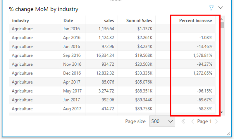
Use case 2: Let’s now calculate the percentage increase in sales month-over-month per industry within a calendar year. We can achieve this by using the percentDifference function. This function calculates percent variance in a metric compared to the previous or following metric, sorted and partitioned by the set of specified dimensions.

percentDifference(aggregated measure, [sort attribute ASC/DESC, ...], -1 or 1, [partition by attribute, ...])

In this formula, the -1 or 1 value indicates whether the difference should be calculated on the preceding or succeeding values respectively. Plugging in the required fields, we arrive at the formula following.

percentDifference(sum(sales),[Date ASC],-1,[industry, truncDate("YYYY",Date)])

If you want only the difference, use the difference function.

difference(aggregated measure, [sort attribute ASC/DESC, ...], lookup index -1 or 1, [partition by attribute, ...])

Availability

Table calculations are available in both Standard and Enterprise editions, in all supported AWS Regions. For more information, see the Amazon QuickSight documentation.

About the Author

Sahitya Pandiri is a technical program manager with Amazon Web Services. Sahitya has been in the product/program management for 5 years now, and has built multiple products in the retail, healthcare and analytics spaces. She enjoys problem solving, and leveraging technology to simplify processes.