AWS for Industries
Predicting the failure of turbofan engines using SpeedWise Machine Learning.
1. Introduction
Equipment failure imposes an enormous burden on industry. It is estimated that unplanned downtime reduces plant productive capacity by between 5 and 20 percent and costs industrial manufacturers $50 billion annually. The cost to repair or replace equipment may be significant, but the true cost of unplanned equipment failure is its consequences. The effects of a failed machine ripple through disrupted downstream operations and heighten exposure to safety hazards and subsequent failures.
Machine lifetime can be extended, and the costs of unanticipated failure can be mitigated by an efficient maintenance strategy. In a cross-sector survey of more than 450 companies, more than 70 percent reported they lacked awareness of when equipment was due for maintenance. A common solution is to routinely replace parts and service equipment at planned intervals. However, all maintenance incurs cost, and routine tasks may be wasteful if performed when they are not warranted. In contrast, predictive maintenance seeks to target maintenance to need by using data-driven analysis to assess equipment condition.
In this post, we will build a machine learning model to address a predictive maintenance task. We will demonstrate how the application of SpeedWise ML (a commercial AutoML solution) can be used to predict the remaining useful life (RUL) of turbofan jet engines. The objective is to quickly propose a predictive model that, using sensor information describing the engine’s present and past performance, can forecast how many timesteps remain until the engine will fail. When applied to a fleet of engines, the model could help the operator’s direct maintenance to those engines most prone to failure, improving the efficiency of a maintenance routine and, most importantly, the fleet’s reliability.
2.1 Problem Description
Turbofan engines are a kind of engine widely used in aircraft propulsion. The average engine operates for 206 cycles. Knowing this, an operator could schedule maintenance every 200 cycles. However, engine lifetimes vary significantly owing to differing:
- Durations of operation
- Settings, intensities, and manners of operation
- Deficiencies particular to a specific machine that may have arisen during component manufacture
In Figure 1, we observe there is a significant spread in engine lifetimes with a minimum and maximum of 128 and 362 cycles, respectively. It is evident a one-size-fits-all maintenance routine based on averages will be inadequate. Can we do better?

Figure 1. The distribution of engine lifetimes in NASA’s FD001 dataset. Engine lifetimes differ so that a one-size-fits-all maintenance approach is inefficient.
To further the development of machine learning solutions to predictive maintenance tasks, NASA’s Prognostic Center of Excellence provides synthetic data on 100 turbofan engines. In the simulated environment, an operator has equipped each engine with 23 sensors that they believe contribute information regarding their health. In Figure 2, we present a few sensor readings for two units that have been run till failure. From this plot alone you might have some intuition about how to engineer features that flag imminent failure. For instance, the gradients of sensors 2–4 trend positive as a fault grows.
An expert might offer more insight still. One might suggest we should check the volatility of a sensor in a recent window. Another might suggest that the interaction of two sensors serves as a leading indicator of failure many cycles in advance. It is easy to see how as the number of timeseries and the sophistication of the prediction task grows, so too does the challenge of identifying these patterns of interest. Hiring an expert to manually condense their knowledge through meticulous feature engineering is time-consuming, expensive, and bound to be nonexhaustive. Instead, machine learning provides a data-driven solution. By feeding many examples of the system’s past behavior into a model, we can train it to recognize the trends in sensor readings that signal engine failure.
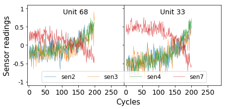
Figure 2. A sample of sensor readings for two engines that have been run till failure.
2.2 What am I looking to accomplish with machine learning?
Machine learning helps us in two ways.
- In a process called timeseries encoding, we will automatically extract hundreds of statistical properties from each sequence. These properties serve as summaries replacing an otherwise hard-to-comprehend timeseries with a succinct but highly informative representation. In addition, the same properties are calculated over window sizes of various lengths. Some will be calculated using only the most recent sensor readings; others will dig deeper into history. This makes encoding robust to signals that manifest over different time scales. By cherry-picking only the most informative statistical properties and systematically calculating them over different timespans, timeseries encoding saves us the burden of manual feature engineering.
- We will then build a model that consumes the encoded sensor representation and outputs a single prediction of the unit’s remaining useful life (the number of operational cycles left until the engine will fail). By feeding a model many examples of input-output pairs, we train it to learn a strategy for mapping from the input to the output space, in this case sensor readings to RUL. Ultimately, when we action our model on new engines for which the RUL is unknown, the model will use this mapping to furnish predictions.
2.3 How SpeedWise ML predicts engine failure
The greater the problem complexity of a machine learning task, the more computational resources tend to be required. We encounter computational bottlenecks in timeseries encoding and model selection. During timeseries encoding, we must calculate hundreds of statistical properties per sequence. During model selection, we must explore hundreds of modeling decisions to arrive at a configuration that optimizes model performance. SpeedWise ML (SML), our code-free AutoML solution of choice, harnesses AWS cloud-distributed computing to make these tasks efficient (Figure 3).
- During timeseries encoding, SML uses AWS Lambda, a serverless compute service apt for small, readily scalable operations. The sequences are distributed across multiple Lambda functions that crunch statistical properties in parallel before assembling them in our final training set.
- During model selection, SML uses an Auto Scaling group of Amazon EC2 instances suited to the compute-intensive demands of model training. In model selection, we explore hundreds of variations in model settings (called hyperparameters), choosing the configuration that yields the best fit across held-out validation folds. SML stages these jobs in an SQS queue, and the Auto Scaling EC2 group executes them in parallel.
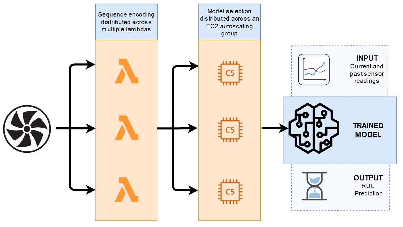
Figure 3. Cloud distributed computing using AWS.
In Table 1, we review the results of frequently cited papers and compare them to SML. We evaluate performance using root-mean-square error (RMSE), a metric that summarizes the discrepancy between model predictions and observations. In this case, the technology found, with little effort, a model that can predict remaining useful life with a 15.22 RMSE. Though SML’s timeseries encoding strategy is very simple and quick to employ, it yields performance competitive with papers that merited scientific publication. Many of those papers employ deep learning models whose architecture is typically time-consuming to define and that typically take an experienced data scientist to tune.
| Method | Test RMSE |
| CNN + FNN | 18.45 |
| SML Timeseries Encoding | 15.22 |
| Time Window Based NN | 15.16 |
| Multi-objective deep belief networks ensemble | 15.04 |
| CNN + FNN without rectified labels | 13.32 |
Table 1. Comparison with state-of-the-art deep learning architectures
SpeedWise ML provides several tools to gain insight into a model. Of particular interest here is the uncertainty quantification plot, which uses a grey band to illustrate confidence in predictions and can help to inform decisions that are robust to noise (Figure 4). For example, we might observe that an engine is forecast to operate for 50 more cycles, but there is a 10 percent chance that it will fail after merely 30. By scheduling maintenance on the engine in the next 30 cycles, an operator can be 90 percent certain that maintenance will pre-empt equipment failure.
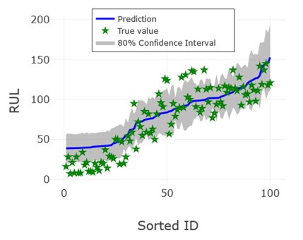
Figure 4. Uncertainty quantification plot for test dataset.
These results show that highly accurate predictive models can be easily obtained by applying smart built-in automated capabilities of commercial machine learning software.
Also, there are opportunities to improve performance even further through:
- Data augmentation. Each timeseries can be strategically chopped up multiple times, serving as examples of an engine at varying states of degradation.
- Preprocessing operations. By smoothing timeseries, we can iron out some of the noise in sensor readings.
- Target transformation. Beyond a threshold, it can be too early in an engine’s lifecycle to detect a fault. This is the motivation for estimating the target using a constant value (130 cycles is often suggested) when the engine is operating normally.
3. Conclusion
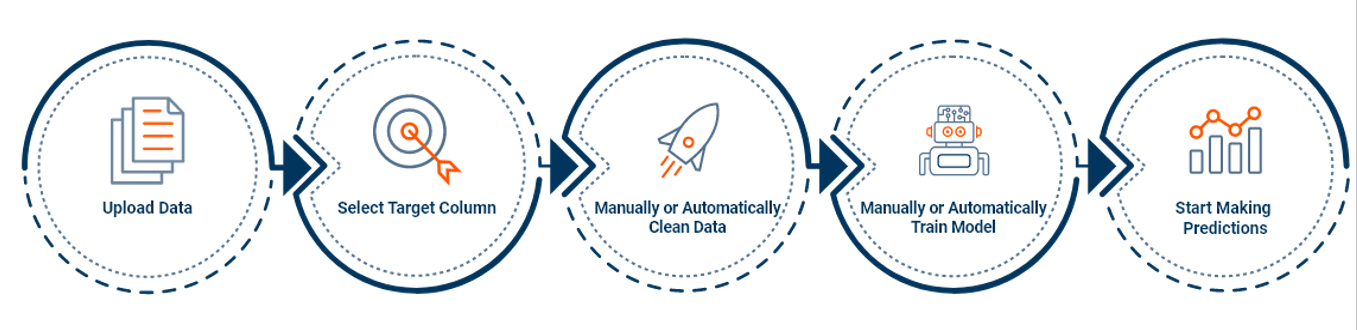
Generating accurate machine learning models for high-impact problems like failure prediction is not a difficult task if the right tools or technologies are used. In this case, SpeedWise ML (Figure 5), an AutoML solution that leverages cloud-computing capabilities, has been used to solve a regression problem estimating the remaining useful life of turbofan jet engines. Typically, interpreting engine sensors might prove challenging. To accurately forecast failure, we must consider not only present but past sensor readings as well. We utilized SML’s timeseries encoder to extract information from each sensor and replace them with a succinct representation apt for model training.