Artificial Intelligence
Next generation Amazon SageMaker Experiments – Organize, track, and compare your machine learning trainings at scale
Today, we’re happy to announce updates to our Amazon SageMaker Experiments capability of Amazon SageMaker that lets you organize, track, compare and evaluate machine learning (ML) experiments and model versions from any integrated development environment (IDE) using the SageMaker Python SDK or boto3, including local Jupyter Notebooks.
Machine learning (ML) is an iterative process. When solving a new use case, data scientists and ML engineers iterate through various parameters to find the best model configurations (aka hyperparameters) that can be used in production to solve the identified business challenge. Over time, after experimenting with multiple models and hyperparameters, it becomes difficult for ML teams to efficiently manage model runs to find the optimal one without a tool to keep track of the different experiments. Experiment tracking systems streamline the processes to compare different iterations and helps simplify collaboration and communication in a team, thereby increasing productivity and saving time. This is achieved by organizing and managing ML experiments in an effortless way to draw conclusions from them, for example, finding the training run with the best accuracy.
To solve this challenge, SageMaker provides SageMaker Experiments, a fully integrated SageMaker capability. It provides the flexibility to log your model metrics, parameters, files, artifacts, plot charts from the different metrics, capture various metadata, search through them and support model reproducibility. Data scientists can quickly compare the performance and hyperparameters for model evaluation through visual charts and tables. They can also use SageMaker Experiments to download the created charts and share the model evaluation with their stakeholders.
With the new updates to SageMaker Experiments, it is now a part of the SageMaker SDK, simplifying the data scientist work and eliminating the need to install an extra library to manage multiple model executions. We are introducing the following new core concepts:
- Experiment: A collection of runs that are grouped together. An experiment includes runs for multiple types that can be initiated from anywhere using the SageMaker Python SDK.
- Run: Each execution step of a model training process. A run consists of all the inputs, parameters, configurations, and results for one iteration of model training. Custom parameters and metrics can be logged using the
log_parameter,log_parameters, andlog_metricfunctions. Custom input and output can be logged using thelog_filefunction.
The concepts that are implemented as part of a Run class are made available from any IDE where the SageMaker Python SDK is installed. For SageMaker Training, Processing and
Transform Jobs, the SageMaker Experiment Run is automatically passed to the job if the job is invoked within a run context. You can recover the run object using load_run() from your job. Finally, with the new functionalities’ integration, data scientists can also automatically log a confusion matrix, precision and recall graphs, and a ROC curve for classification use cases using the run.log_confusion_matrix, run.log_precision_recall, and run.log_roc_curve functions, respectively.
In this blog post, we will provide examples of how to use the new SageMaker Experiments functionalities in a Jupyter notebook via the SageMaker SDK. We will demonstrate these capabilities using a PyTorch example to train an MNIST handwritten digits classification example. The experiment will be organized as follow:
- Creating experiment’s runs and logging parameters: We will first create a new experiment, start a new run for this experiment, and log parameters to it.
- Logging model performance metrics:We will log model performance metrics and plot metric graphs.
- Comparing model runs:We will compare different model runs according to the model hyperparameters. We will discuss how to compare those runs and how to use SageMaker Experiments to select the best model.
- Running experiments from SageMaker jobs: We will also provide an example of how to automatically share your experiment’s context with a SageMaker processing, training or batch transform job. This allows you to automatically recover your run context with the
load_runfunction inside your job. - Integrating SageMaker Clarify reports: We will demonstrate how we can now integrate SageMaker Clarify bias and explainability reports to a single view with your trained model report.
Prerequisites
For this blog post, we will use Amazon SageMaker Studio to showcase how to log metrics from a Studio notebook using the updated SageMaker Experiments functionalities. To execute the commands presented in our example, you need the following prerequisites:
- SageMaker Studio Domain
- SageMaker Studio user profile with SageMaker full access
- A SageMaker Studio notebook with at least an
ml.t3.mediuminstance type
If you do not have a SageMaker Domain and user profile available, you can create one using this quick setup guide.
Logging parameters
For this exercise, we will use torchvision, a PyTorch package that provides popular datasets, model architectures, and common image transformations for computer vision. SageMaker Studio provides a set of Docker images for common data science use cases that are made available in Amazon ECR. For PyTorch, you have the option of selecting images optimized for CPU or GPU training. For this example, we will select the image PyTorch 1.12 Python 3.8 CPU Optimized and the Python 3 kernel. The examples described below will focus on the SageMaker Experiments functionalities and are not code complete.
Let’s download the data with the torchvision package and track the number of data samples for the train and test datasets as parameters with SageMaker Experiments. For this example, let’s assume train_set and test_set as already downloaded torchvision datasets.
In this example, we use the run.log_parameters to log the number of train and test data samples and run.log_file to upload the raw datasets to Amazon S3 and log them as inputs to our experiment.
Training a model and logging model metrics
Now that we’ve downloaded our MNIST dataset, let’s train a CNN model to recognize the digits. While training the model, we want to load our existing experiment run, log new parameters to it, and track the model performance by logging model metrics.
We can use the load_run function to load our previous run and use it to log our model training
We can then use run.log_parameter and run.log_parameters to log one or multiple model parameters to our run.
And we can use run.log_metric to log performance metrics to our experiment.
For classification models, you can also use run.log_confusion_matrix, run.log_precision_recall, and run.log_roc_curve, to automatically plot the confusion matrix, precision recall graph, and the ROC curve of your model. Since our model solves a multiclass classification problem, let’s log only the confusion matrix for it.
When looking at our run details, we can now see the generated metrics as shown in the screenshot below:
The run details page provides further information about the metrics.
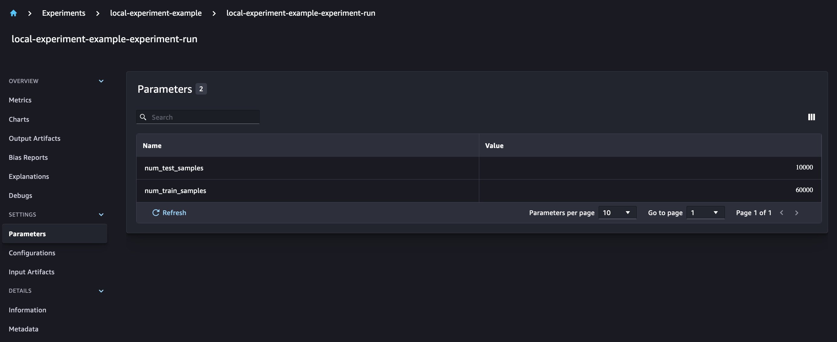
And the new model parameters are tracked on the parameters overview page.
You can also analyze your model performance by class using the automatically plotted confusion matrix, which can also be downloaded and used for different reports. And you can plot extra graphs to analyze the performance of your model based on the logged metrics.
Comparing multiple model parameters
As a data scientist, you want to find the best possible model. That includes training a model multiple times with different hyperparameters and comparing the performance of the model with those hyperparameters. To do so, SageMaker Experiments allows us to create multiple runs in the same experiment. Let’s explore this concept by training our model with different num_hidden_channels and optimizers.
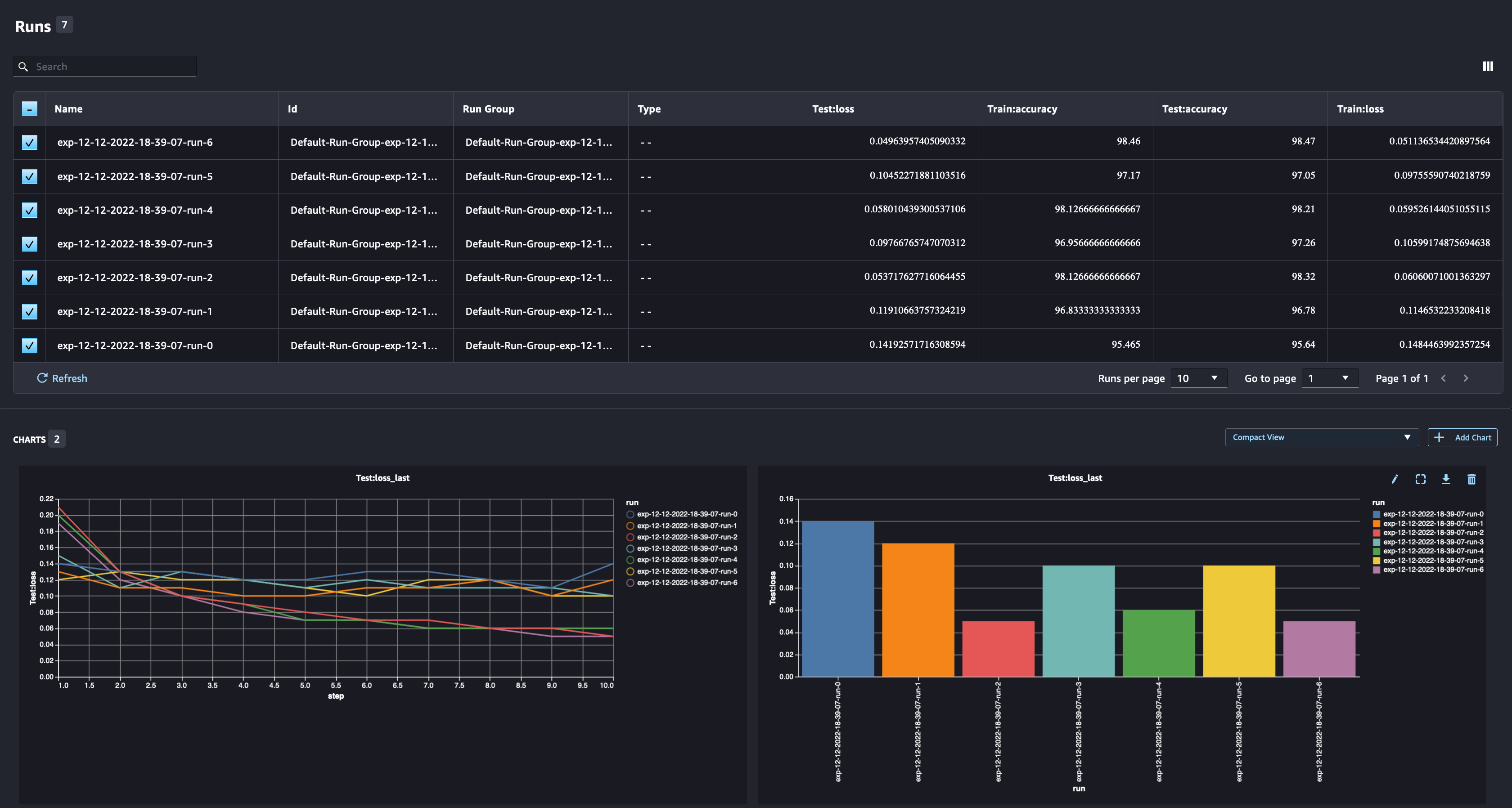
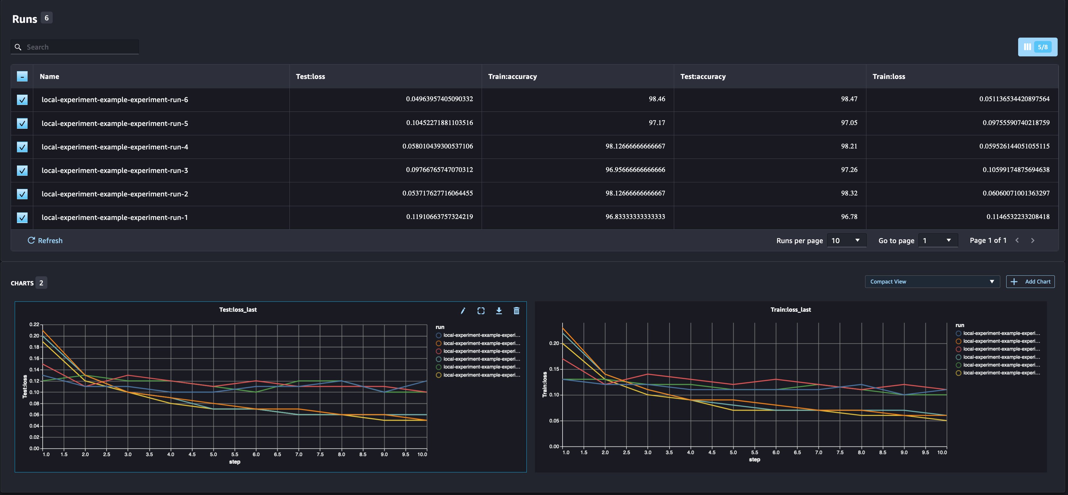
We are now creating six new runs for our experiment. Each one will log the model parameters, metrics, and confusion matrix. We can then compare the runs to select the best-performing model for the problem. When analyzing the runs, we can plot the metric graphs for the different runs as a single plot, comparing the performance of the runs across the different training steps (or epochs).
Using SageMaker Experiments with SageMaker training, processing and batch transform jobs
In the example above, we used SageMaker Experiments to log model performance from a SageMaker Studio notebook where the model was trained locally in the notebook. We can do the same to log model performance from SageMaker processing, training and batch transform jobs. With the new automatic context passing capabilities, we do not need to specifically share the experiment configuration with the SageMaker job, as it will be automatically captured.
The example below will focus on the SageMaker Experiments functionalities and is not code complete.
In our model script file, we can get the run context using load_run(). In SageMaker processing and training jobs, we do not need to provide the experiment configuration for loading the configuration. For batch transform jobs, we need to provide experiment_name and run_name to load the experiment’s configuration.
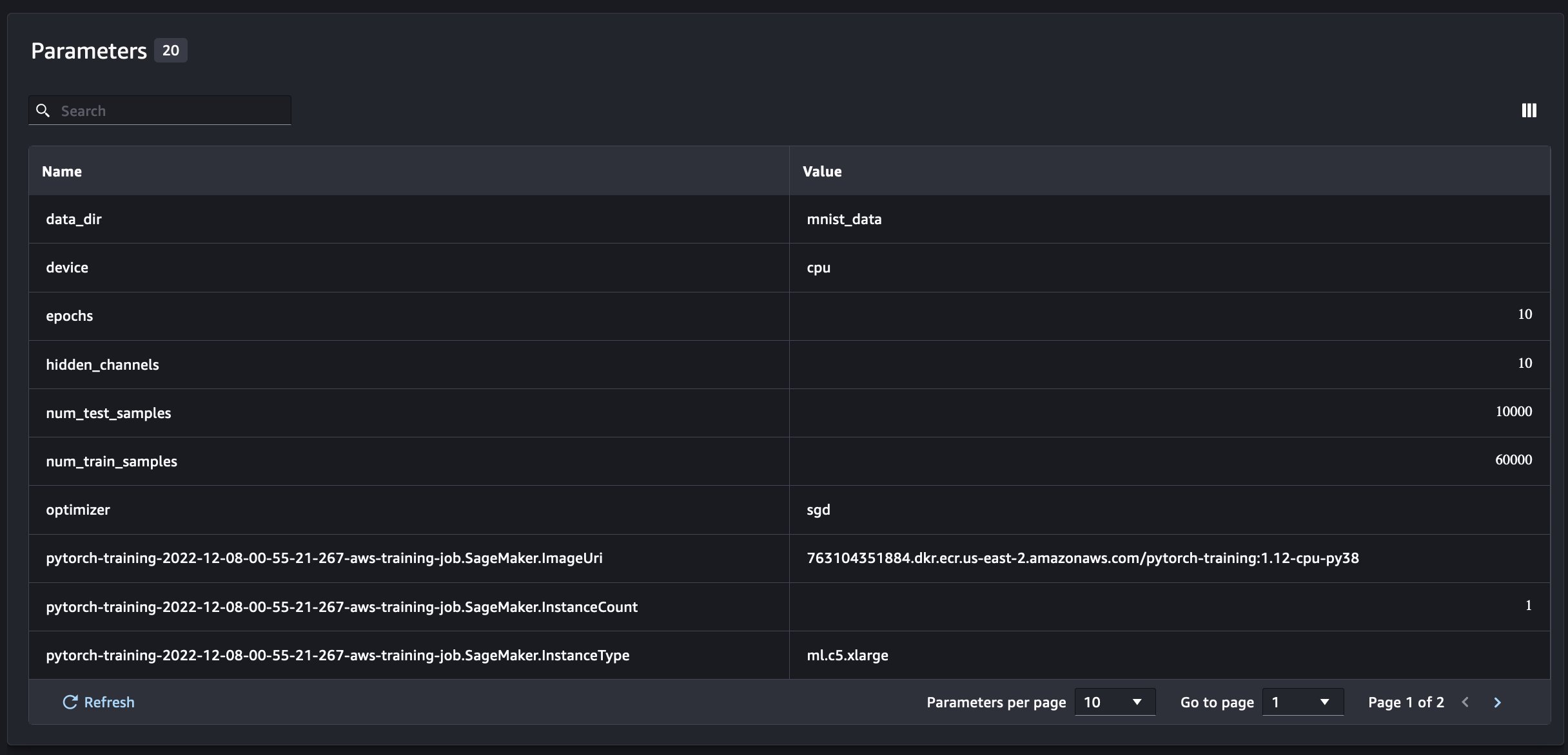
In addition to the information we get when running SageMaker Experiments from a notebook script, the run from a SageMaker job will automatically populate the job parameters and outputs.
The new SageMaker Experiments SDK also ensures backwards compatibility with the previous version using the concepts of trials and trial components. Any experiment triggered using the previous SageMaker Experiments version will be automatically made available in the new UI, for analyzing the experiments.
Integrating SageMaker Clarify and model training reports
SageMaker Clarify helps improve our ML models by detecting potential bias and helping explain how these models make predictions. Clarify provides pre-built containers that run as SageMaker processing jobs after your model has been trained, using information about your data (data configuration), model (model configuration), and the sensitive data columns that we want to analyze for possible bias (bias configuration). Up until now, SageMaker Experiments displayed our model training and Clarify reports as individual trial components that were connected via a trial.
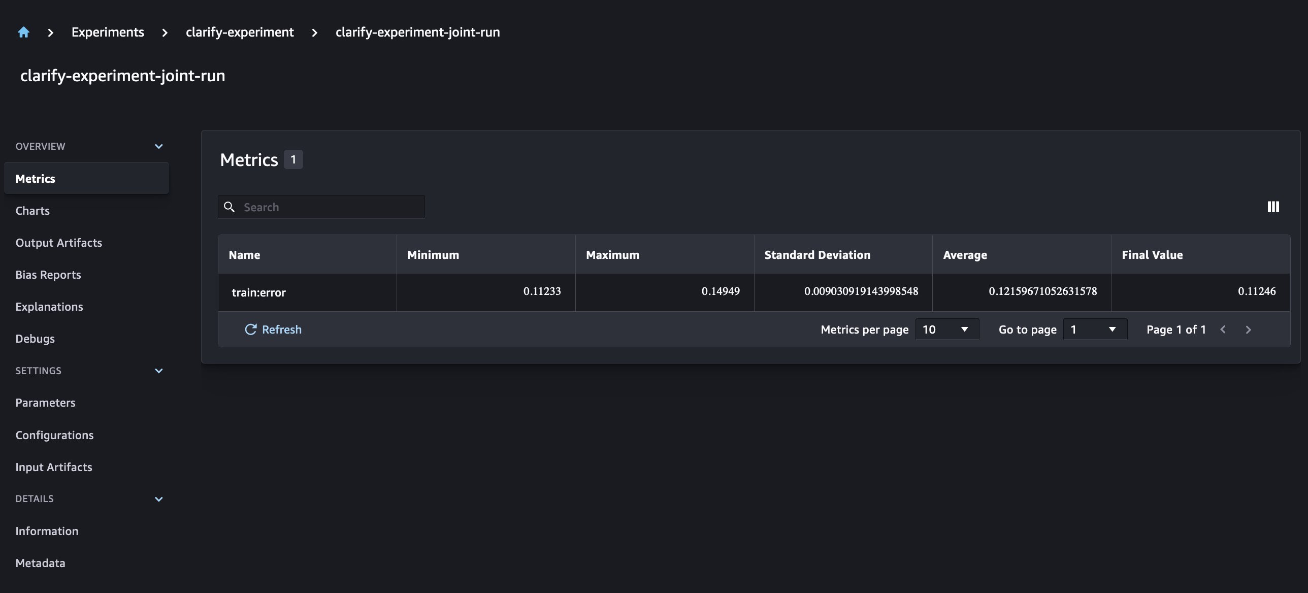
With the new SageMaker Experiments, we can also integrate SageMaker Clarify reports with our model training having one source of truth that allows us to further understand our model. For an integrated report, all we need to do is to have the same run name for our training and Clarify jobs. The following example demonstrates how we can integrate the reports using an XGBoost model to predict the income of adults across the United States. The model uses the UCI Adult dataset. For this exercise, we assume that the model was already trained and that we already calculated the data, model, and bias configurations.
With this setup, we get a combined view that includes the model metrics, joint inputs and outputs, and the Clarify reports for model statistical bias and explainability.
Conclusion
In this post, we explored the new generation of SageMaker Experiments, an integrated part of SageMaker SDK. We demonstrated how to log your ML workflows from anywhere with the new Run class. We presented the new Experiments UI that allows you to track your experiments and plot graphs for a single run metric as well as to compare multiple runs with the new analysis capability. We provided examples of logging experiments from a SageMaker Studio notebook and from a SageMaker Studio training job. Finally, we showed how to integrate model training and SageMaker Clarify reports in a unified view, allowing you to further understand your model.
We encourage you to try out the new Experiments functionalities and connect with the Machine Learning & AI community if you have any questions or feedback!
About the Authors
 Maira Ladeira Tanke is a Machine Learning Specialist at AWS. With a background in Data Science, she has 9 years of experience architecting and building ML applications with customers across industries. As a technical lead, she helps customers accelerate their achievement of business value through emerging technologies and innovative solutions. In her free time, Maira enjoys traveling and spending time with her family someplace warm.
 Mani Khanuja is an Artificial Intelligence and Machine Learning Specialist SA at Amazon Web Services (AWS). She helps customers using machine learning to solve their business challenges using the AWS. She spends most of her time diving deep and teaching customers on AI/ML projects related to computer vision, natural language processing, forecasting, ML at the edge, and more. She is passionate about ML at edge, therefore, she has created her own lab with self-driving kit and prototype manufacturing production line, where she spends lot of her free time.
 Dewen Qi is a Software Development Engineer at AWS. She currently participating in building a collection of platform services and tools in AWS SageMaker to help customer in making their ML projects successful. She is also passionate about bringing the concept of MLOps to broader audience. Outside of work, Dewen enjoys practicing Cello.
 Abhishek Agarwal is a Senior Product Manager for Amazon SageMaker. He is passionate about working with customers and making machine learning more accessible. In his spare time, Abhishek enjoys painting, biking and learning about innovative technologies.
 Dana Benson is a Software Engineer working in the Amazon SageMaker Experiments, Lineage, and Search team. Prior to joining AWS, Dana spent time enabling smart home functionality in Alexa and mobile ordering at Starbucks.

