A detailed, end-to-end assessment of a quantum algorithm for portfolio optimization, released by Goldman Sachs and AWS

To date, the financial services industry has been a pioneer in quantum technology, owing to its plethora of computationally hard use cases and the potential for significant impact from quantum solutions. Daily operations at financial firms such as banks, insurance companies, and hedge funds require solving well-defined computational problems on underlying data that is constantly changing. If quantum computers can perform the same calculations faster or with better accuracy than existing solutions, these customers stand to reap significant benefit.

In this post we’ll walk you through some key takeaways from a body of work by scientists from Goldman Sachs and AWS that was published today in the journal PRX Quantum [1].

Background

A commonly studied use case in quantitative finance is the task of portfolio optimization — consequently, customers are eager to learn what impacts quantum computing can have on this task, if any. Several distinct quantum algorithms have been proposed for portfolio optimization, each of which leverage quantum effects to provide a theoretical speedup over comparable classical algorithms.

However, it has been difficult to assess whether these theoretical speedups can be realized in practice. Such an assessment requires an end-to-end resource estimation of the quantum algorithm — that is, a calculation of the total number of qubits and quantum gates (or other relevant metrics) required to solve the actual problem of interest, without sweeping any costs or caveats under the rug.

End-to-end assessments are challenging because certain elements of the quantum algorithm are heuristic, and there are caveats related to the way the quantum computer accesses the data. Thus, it can be difficult to make apples-to-apples comparisons with existing methods

Despite the challenges, scientists from Goldman Sachs and AWS took on the task of performing an end-to-end resource estimate for a leading quantum approach to portfolio optimization — the quantum interior point method (QIPM), which we will discuss in this post. You can read the full paper in the journal PRX Quantum, but let’s walk through some of the main takeaways of that work [1].

How do we determine if a quantum algorithm is practical?

For quantum computers to provide value over classical algorithms, we need to develop practical, end-to-end quantum algorithms, for which we identify the following criteria:

1. The quantum algorithm produces a classical output that allows for benchmarking against classical methods. This requirement rules out some quantum “algorithms” that efficiently produce quantum states as output, but are much less efficient when forced to turn that quantum state into an answer to the original (classical) computational problem.
2. The quantum algorithm relies on a reasonable input model. In particular, it does not utilize any unspecified black-box subroutines (often called “oracles”) for which the costs are not counted, nor does it assume fast data access without accounting for the true cost of quantum access to the classical data. For example, several quantum algorithms for Machine Learning were thought to offer exponential advantages over classical methods until it was pointed out that this was primarily an artifact of unreasonable assumptions about the input model [2].
3. The quantum algorithm has a plausible case for asymptotic quantum speedup — that is, for sufficiently large instance sizes, the quantum algorithm requires substantially fewer elementary operations than the classical algorithm. Since classical computers can perform elementary operations at a much faster rate than quantum computers, without an asymptotic speedup, the quantum computer will always lose.
4. For classically challenging problem sizes, the quantum algorithm can solve the same end-to-end problem in a reasonable run-time. Asymptotic speedups are of no value if the crossover point where quantum computers outperform classical computers occurs at instance sizes that are too large to be useful to customers.

Portfolio optimization

Portfolio optimization is a well-defined computational task that appears in many fields, but its utility is particularly clear for financial operations. Suppose you have a fixed budget to invest in the stock market. You’d like your investments to provide predictable growth; in particular, you’d like to construct a portfolio that maximizes the expected return of the portfolio, while minimizing the risk, that is, the amount by which the return might deviate from its expectation.

The model

Part of the problem is thus determining which stocks are expected to perform well in a given timeframe, based on historical data — we assume this has already been done. If there are n stocks to invest in, we are provided as input with a length-n vector containing the expected return for each of the stocks, as well as an n x n matrix 𝛴 containing the historical volatilities of each stock and the covariance of each pair of stocks — the performance of different stocks is correlated, and the optimal portfolio will exploit these correlations to minimize portfolio risk.

Let w be the length-n vector representing the fraction of our budget we allocate to each stock. In general, entries of w can be negative, which represents a short sale. Here, though, we will require that the portfolio contain only “long” assets — i.e., no short sales: w_i ≥ 0. The portfolio optimization problem is then formulated as a convex optimization problem:

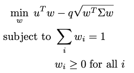
The parameter q is called the “risk-aversion parameter”, and it is set by the user according to how much risk they are willing to take on to gain additional return.

The first constraint is a total budget constraint. We’ve normalized w so that the total budget available is just 1, but without normalizing this sum would equal the total amount of money available to invest.

The second constraint enforces the “long-only” condition above; if we allow short selling, this can be relaxed. Additional constraints, such as minimum or maximum investments in certain stock sectors, cardinality constraints (i.e., the maximum allowed number of assets), or transaction costs, can also be incorporated into this framework (see [3]).

The set of portfolios that obey all the constraints is known as the feasible region. The feasible region can be divided into the boundary, where at least one of the inequality constraints holds as an equality (e.g. w_i = 0), and the interior, where all inequality constraints are strict (w_i > 0 for all i).

One widely used classical approach for solving portfolio optimization is to map the convex optimization problem above to a type of optimization problem known as a second-order cone program (SOCP), and then solve it with an interior point method (IPM). The basic idea of an IPM is to start at some portfolio in the interior of the feasible region and iteratively update it in a way that is guaranteed to eventually approach the optimal portfolio, which lies on the boundary of the feasible region, as depicted in Figure 1.

Figure 1: A toy example depicting how an Interior Point Method (IPM) solves portfolio optimization. The hexagonal region represents the feasible set of portfolios. The IPM generates a sequence of points (known as the central path) that follows a path from the interior of the region to the optimal point, which lies on the boundary. The color represents the value of the objective function, including barrier functions that implement constraints (darker is better). The black dots represent the central path, which is defined to be the optimal point of the objective function, including the barrier. As the barrier functions are relaxed, the objective function approaches the true objective function, and the central path approaches the optimal solution to the problem on the boundary of the feasible space.

Performing a single iteration of the IPM requires solving a linear system of equations of size L x L, where (in our formulation), L ≈ 14n and n is the number of stocks in which we could invest. The output of the IPM is a portfolio w that obeys all the constraints and for which the objective function is within 𝜖 of the optimal value. Many flavors of IPM exist, and developing better classical IPMs is an active area of research.

Here we focus on the IPMs that are most comparable with quantum algorithms. These classical IPMs solve the PO problem in time scaling as n^3.5 log(1/𝜖). This runtime is efficient in theory (i.e., it scales polynomially with n) and also in practice (IPMs are a leading method underlying many open-source and commercial solvers). Using IPM-based, off-the-shelf solvers, one can solve the PO problem on portfolios with thousands of stocks reasonably quickly on standard compute resources. However, the n^3.5 scaling is steep, and pushing the number of assets into the tens of thousands presents an opportunity for alternative solutions (such as quantum computing) to provide value. In the next section, we explore a proposal to do exactly that.

Quantum interior point methods

Quantum interior point methods (QIPMs) aim to accelerate classical IPMs by replacing certain algorithmic steps with quantum subroutines. The fact that IPMs are efficient both in theory and in practice gives hope that, if indeed these subroutines can be completed more quickly, QIPMs could satisfy the four criteria of a practical quantum algorithm and deliver practical utility in customer use cases.

QIPMs preserve the main loop of the IPM (which iteratively generates a sequence of better and better portfolios), and replaces a subroutine in the IPM that solves linear systems of equations with a quantum algorithm for completing this task. To do this, QIPMs leverage three quantum ingredients — Quantum Random Access Memory, quantum linear system solvers, and quantum state tomography — in each iteration of the main loop. These ingredients perform the following roles:

• Quantum Random Access Memory (QRAM) allows the quantum algorithm to access the data that defines the instance, namely u and 𝛴, in an efficient and quantum mechanical way. Theoretical analyses of QRAM-based algorithms often merely report the number of queries to the QRAM data structure and assume the query time is very fast. To account for criterion 2 (reasonable input model), a full end-to-end analysis must go further and compute the exact resources required to perform the QRAM queries. Specifically, our resource analysis for the QIPM utilizes the resource estimates for implementing a block-encoding of an arbitrary matrix — a primitive that is in some sense equivalent to QRAM — that we developed in separate, parallel work [4].
• Quantum linear system solvers (QLSSs), as their name suggests, are quantum subroutines for solving linear systems of the form Ax = b, where A is an invertible L x L matrix, and x and b are length-L vectors. In the PO problem, L ≈ 14n. The catch is that, unlike classical linear system solvers, QLSSs do not output the vector x; rather, they output a quantum state |x⟩ whose amplitudes are proportional to the entries of x.
• Quantum state tomography is precisely the subroutine that turns the quantum state |x⟩ into a classical description of the vector x, which is then used to iterate the IPM. In essence, tomography is performed just by preparing many copies of |x⟩, measuring them, and gathering statistics on the frequency of each measurement outcome to estimate the entries of x. The need for tomography is related to criterion 1, above; the QLSS is efficient, but it outputs a quantum state rather than classical data, and this quantum state is not the object that is immediately useful to the rest of the algorithm.

The full end-to-end analysis takes care to account for errors incurred by each of these primitive ingredients. The largest of these errors is incurred by tomography, due to the statistical noise of estimating an entry of x from measurement outcomes of |x⟩. An additional caveat is that these small errors prevent the QIPM from exactly following the same path as the classical IPM, and they also cause the QIPM to leave the feasible region. Luckily, the IPM is designed to be self-correcting, in the sense that it partially fixes any errors it makes in future iterations.

Ultimately, through this effect or other workarounds we explore in the full paper, the QIPM will solve the same problem as the classical IPM: it returns an ϵ-optimal solution in an amount of time that essentially scales as:

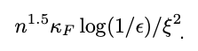
The appearance of new parameters ⲕ_F and ξ represent additional technical complications, and need to be unpacked. The parameter ⲕ_F is the “Frobenius condition number” — it represents the difficulty of inverting the relevant matrices with the QLSS. The parameter ξ is the maximum error on quantum state tomography that does not break the algorithm (i.e., how poorly we can estimate the state |x⟩) — small errors are okay as long as subsequent iterations of the IPM find portfolios that are close enough to those of an ideal IPM.

These are instance-specific parameters, meaning that two different instances of the PO problem with stocks will have different values for ⲕ_F and ξ, which makes the magnitude and scaling of these parameters difficult to study. This is an issue, because it is clear that the effectiveness of the algorithm critically hinges on how large they are! If ⲕ_F and 1/ξ are small and constant, one is tempted to declare that the quantum algorithm has a large n^3.5 → n^1.5 speedup over the classical IPM. However, it is expected that these parameters will also have an n dependence, cutting into this speedup. Work by Kerenidis, Prakash, and Szilágyi [5] studied one version of the QIPM for portfolio optimization and gave some preliminary numerical evidence that the QIPM still offers a speedup after accounting for the dependence on ⲕ_F and ξ.

The expression above omits some additional logarithmic factors: we computed the full expression of the runtime to be proportional to:

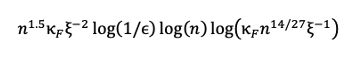
These log factors are typically ignored in asymptotic analyses (such as that of Kerenidis, Prakash, and Szilágyi [5]), where the goal is to judge criterion 3 of a practical end-to-end algorithm, as these factors have a relatively small contribution in the limit where n and other parameters are large. However, to judge criterion 4, it is essential to keep track of all contributions, as they can make a big difference on the runtime estimate for specific choices of n.

Resource estimate for the QIPM

To judge criterion 4, we need to know how many quantum resources the QIPM consumes for values of n relevant to customers. We compute the number of logical qubits, the number of computationally expensive T gates (i.e., the “T-count”), and the number of layers of T gates (i.e., “T-depth”) required by the algorithm. A T gate is a commonly studied quantum gate that, when coupled with other easy-to-implement quantum gates, equips quantum computers with their expressive power. We only count the T gates because they are substantially more expensive than the other gates in popular approaches to fault-tolerant quantum computation, and they dominate the runtime of the algorithm. The number of logical qubits and the total number of T gates are then used to determine the overall physical footprint of the quantum algorithm — this will also depend on details of the physical hardware, such as the physical error rate.

Meanwhile, the T-depth determines the runtime in an architecture where T-gates on disjoint qubits can be implemented in parallel. These metrics have been computed for other quantum algorithms, allowing for reasonable comparisons.

For a version of the PO problem like the one above, with a couple of additional, common constraints, we find that optimizing an n-qubit portfolio to tolerance ϵ requires

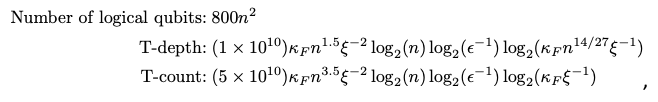
where we omit subleading terms. Notably, the order-n² overhead for the T-count vs. the T-depth, and the order-n² logical qubit dependence reflects the fact that QRAM can be implemented at shallow depth albeit, with large qubit and gate cost.

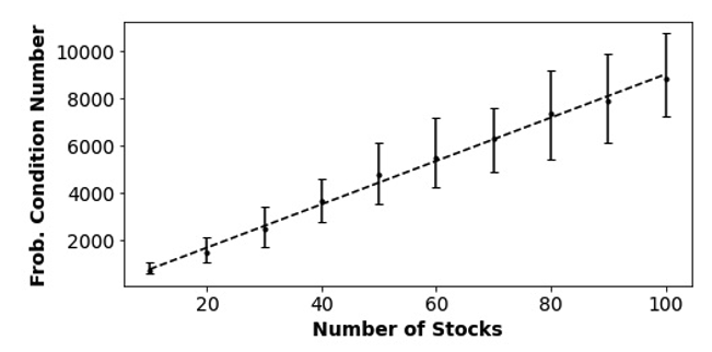
Figure 2: Median value of the Frobenius condition number as a function of the number of stocks in the portfolio optimization instance, from numerical simulations. Error bars represent the 16th to 84th percentile of observed instances, and the dashed line is a power-law fit showing that the growth of the Frobenius condition number is nearly linear in n.

The above expressions are not particularly illuminating, as they still depend on instance-specific parameters ⲕ_F and ξ. To probe these parameters, we simulated random instances of portfolio optimization with n varying from 10 to 120. For each instance, we chose a random set of n stocks from the Dow Jones U.S. Total Stock Market Index (DWCF) and constructed the expected daily return vector u and covariance matrix 𝛴 using historical stock data collected over 2n time epochs. We found that both ⲕ_F and ξ ^-2 appear to grow with n, on average, and were each typically on the order of 10⁴ or 10⁵ for n = 100. Overall, we evaluated the average cost of the algorithm at n=100 to be:

• Number of logical qubits: 8 million
• T-depth: 2 x 10²⁴
• T-count: 7 x 10²⁹

Even if layers of T-gates are optimistically implemented at the GHz speeds of classical processors (in reality they are likely to be 2–4 orders of magnitude slower than that) these estimates suggest that the runtime of the quantum algorithm would still be millions of years, even for an instance size that is already classically tractable on a laptop.

This outcome allows us to confidently say that the QIPM, in its current form, does not satisfy criterion 4 of the end-to-end practical algorithm. The reason this occurred was due to a confluence of several independent factors: a large constant pre-factor coming mainly from the QLSS, a large condition number ⲕ_F, a significant number of samples needed for tomography, and even a non-negligible contribution from logarithmic factors (about a factor of 100,000 for the T-depth) that are traditionally ignored in asymptotic analyses.

These estimates also incorporate a few improvements we made to the algorithm, including an adaptive approach to tomography, and preconditioning the linear systems. However, there are several ways one could try to improve the algorithm further, including using newer, more advanced versions of quantum state tomography [6] with ξ^-1 rather than ξ^-2 dependence, additional preconditioning, or improvements to the QLSS. Nonetheless, the resource estimate we arrive at is so far from practicality that multiple improvements to various parts of the algorithm would be needed to make the algorithm practical.

In retrospect, we can also consider whether the algorithm meets criterion 3, i.e., if it has an asymptotic speedup. The numerical simulations of Kerenidis, Prakash, and Szilágyi [5] suggested it does, but our numerical simulations fail to corroborate this, since we find that the scaling of the algorithmic runtime in the regime 10 ≤ n ≤ 120 is roughly the same as the classical algorithm. However, this scaling does not have a robust trend, and cannot confidently extrapolate to larger industrially relevant choices of n.

Conclusion and takeaways

Our end-to-end resource analysis of the QIPM for portfolio optimization is a revealing case study on the utility of quantum algorithms. Even when an algorithm presents signals of utility, closer inspection can reveal a drastically different picture when all factors are considered more fairly. This was the case for the QIPM—our analysis strongly suggests it will not be useful to customers, barring significant improvements to the underlying algorithm. However, the insights gleaned go beyond the QIPM; the core subroutines of the QIPM (QRAM, QLSS, tomography) are common to many other quantum algorithms as well. Parts of our detailed cost analysis could thus be re-utilized in those algorithms. Indeed, one specific lesson learned is the great cost of implementing quantum circuits for the data-access component of the quantum algorithm (QRAM).

The QRAM accounts for most of the logical qubits in our accounting, and contributes a considerable factor to the gate depth and gate count. To improve the QIPM to the point of practicality, one ingredient which would likely be necessary is a dedicated QRAM hardware element that can leverage the specialized, non-universal nature of the QRAM operation to perform the operation more efficiently than our general analysis accounts for. This hardware element would also improve the practicality of many other quantum algorithms in many domains such as quantum machine learning, quantum chemistry, and quantum optimization.

With our analysis revealing that QIPMs face significant challenges toward practicality, where does this leave portfolio optimization in the landscape of quantum computing applications? Fortunately, there are other proposed methods for solving portfolio optimization on quantum computers (e.g., [7]), and some of these are even amenable to near-term experimentation.

These approaches operate by reformulating the convex problem above as a binary optimization problem and attacking them with variational quantum algorithms, such as the quantum approximate optimization algorithm (QAOA), or using specialized hardware such as quantum annealers.

The upshot is that some of these variational approaches can already be run on near-term quantum devices through Amazon Braket, but one loses the theoretical asymptotic success guarantees afforded by the QIPM. As such, it is unclear whether these near-term solutions satisfy the third criterion above (asymptotic speedup), and determining whether this is the case will require further empirical investigation using current hardware and future generations of devices.

Finance remains a rich space for potential quantum algorithms, and perhaps some of the ideas in the QIPM will prove fruitful toward developing practical algorithms in the future. We hope that this example inspires researchers to search for the next generation of innovative, practical quantum algorithms in a systematic, end-to-end way.

References

[1] Alexander M. Dalzell, B. David Clader, Grant Salton, Mario Berta, Cedric Yen-Yu Lin, David A. Bader, Nikitas Stamatopoulos, Martin J. A. Schuetz, Fernando G. S. L. Brandão, Helmut G. Katzgraber, William J. Zeng. “End-to-end resource analysis for quantum interior point methods and portfolio optimization.” PRX Quantum 4, 040325 (2023). https://doi.org/10.1103/PRXQuantum.4.040325

[2] Ewin Tang. “Quantum Principal Component Analysis Only Achieves an Exponential Speedup Because of Its State Preparation Assumptions” Phys. Rev. Lett. 127, 06050 (2021). https://doi.org/10.1103/PhysRevLett.127.060503

[3] “MOSEK Portfolio Optimization Cookbook.“ Release 1.3.0 (2023) https://docs.mosek.com/MOSEKPortfolioCookbook-a4paper.pdf

[4] Blog: “Goldman Sachs and AWS examine efficient ways to load data into quantum computers“
Paper: B. David Clader, Alexander M. Dalzell, Nikitas Stamatopoulos, Grant Salton, Mario Berta, William J. Zeng. “Quantum Resources Required to Block-Encode a Matrix of Classical Data.” IEEE Transactions on Quantum Engineering (Volume: 3) (2022) https://doi.org/10.1109/TQE.2022.3231194.

[5] Iordanis Kerenidis, Anupam Prakash, Dániel Szilágyi. “Quantum Algorithms for Portfolio Optimization.” Proceedings of the 1st ACM Conference on Advances in Financial Technologies. (2019) https://doi.org/10.1145/3318041.3355465

[6] Joran van Apeldoorn, Arjan Cornelissen, András Gilyén, and Giacomo Nannicini. “Quantum tomography using state-preparation unitaries.” Proceedings of the 2023 Annual ACM-SIAM Symposium on Discrete Algorithms (SODA). https://doi.org/10.1137/1.9781611977554.ch47

[7] Sebastian Brandhofer, Daniel Braun, Vanessa Dehn, Gerhard Hellstern, Matthias Hüls, Yanjun Ji, Ilia Polian, Amandeep Singh Bhatia, Thomas Wellens. “Benchmarking the performance of portfolio optimization with QAOA.” Quantum Inf. Process 22, 25 (2023) https://doi.org/10.1007/s11128-022-03766-5