Constructing an “end-to-end” quantum algorithm: a comprehensive technical resource for algorithms designers

Today we are introducing Quantum algorithms: A survey of applications and end-to-end complexities [1]. This is a comprehensive resource, designed for quantum computing researchers and customers who are looking to explore how quantum algorithms will apply to their use cases.

The survey provides a detailed technical analysis of the end-to-end quantum resource requirements (the “complexities”) of the most widely studied quantum computing application areas, like chemistry, finance, and machine learning.

The primary focus of the survey is quantum algorithms with the greatest potential to generate customer value in the long term, once fault-tolerant quantum computers are available – however, it also comments on the most relevant near-term noisy intermediate-scale quantum (NISQ) algorithms, where appropriate.

Background

The ultimate goal of research into quantum computing is to build a quantum computer that is powerful enough to surpass classical computers at useful computational tasks. But how much power is “enough” – and how can you quantify computational power?

To answer these questions, we start by designing a quantum algorithm that solves a concrete customer problem. Running this algorithm on an actual quantum computer would consume quantum resources – measured primarily by the number of qubits and the number of basic quantum operations (gates) required by the algorithm. A calculation of the quantity of these resources needed to fully solve the customer problem is called an end-to-end resource estimate. This estimate can easily be compared to the current status of quantum hardware development – and to existing classical solutions – to evaluate the value proposition of quantum computing for a given industry.

The survey was born out of research at the AWS Center for Quantum Computing. It seeks to aid rapid assessments of quantum applications by capturing the dominant contributions to their resource requirements. It has a modular, wiki-like structure to enable researchers to experiment in a “plug-and-play” fashion – it is easy to see how interchanging different subroutines into a quantum algorithm affects the overall complexity. It is also careful to take into account the caveats and implicit limitations present in many quantum algorithms – including those associated with quantum error correction.

Together with its focus on comparing to best-in-class classical solutions, it aims to provide a realistic, unobscured picture of how quantum computers can one day fit into customer workflows.

Why are we releasing this survey now?

Quantum computing is currently in the “noisy intermediate-scale” era. The devices have (at most) hundreds of physical qubits, and are on the cusp of demonstrating quantum error correction. Nevertheless, a long-lived logical qubit – the basic building block of fault-tolerant quantum algorithms – has not yet been experimentally demonstrated. Existing quantum devices are still orders of magnitude away from the capabilities required to demonstrate large-scale fault-tolerant quantum computation. So what do we hope to achieve by releasing this survey?

For researchers, the disparity between current quantum hardware and resource estimates for quantum algorithms, is a call to action – an invitation to innovate. Every qubit and gate saved by an improved resource estimate reduces the burden on quantum hardware engineers. As researchers who innovate on behalf of our customers, we know firsthand that designing new and improved quantum applications is challenging. In many instances, the required domain expertise and background in quantum algorithms and error correction are scattered throughout the literature. Moreover, one must factor in hidden caveats, and the performance of best-in-class classical approaches. There is often a disconnect between the tasks that quantum computers appear best suited for, and those tasks most relevant to customers. These challenges make it difficult to gather a holistic view of the overall solution and compute an accurate end-to-end resource estimate for practical customer problems.

When analyzing and optimizing quantum algorithms for a range of problems, we found that the most useful insights and pieces of knowledge appeared multiple times in different quantum algorithms and applications. We decided to collect this information in a single location.

We have found that the streamlined, modular structure of the survey has enabled us to quickly understand and analyze new quantum algorithms. We hope that by sharing this survey with the community, other researchers will be empowered to view quantum algorithms in an end-to-end fashion. Ultimately, we hope that this work can grow beyond the research of our own team, and become an important resource for the quantum computing community.

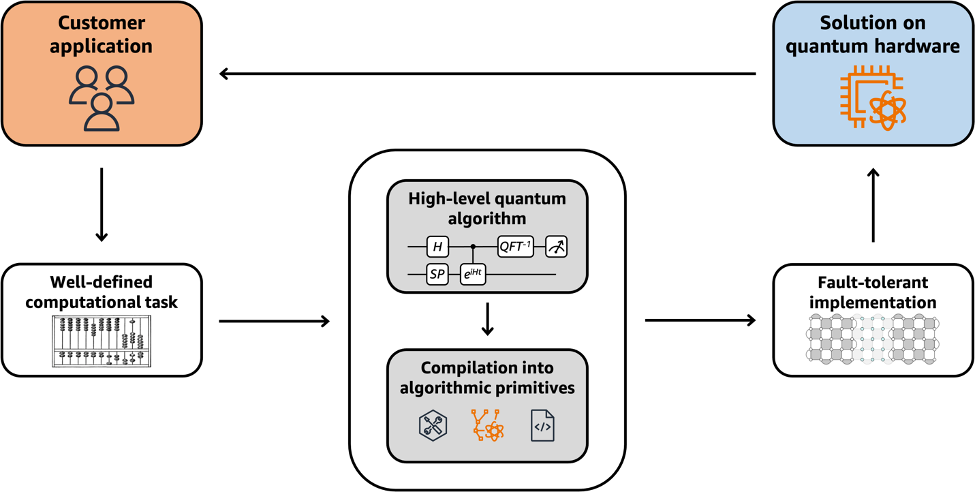
Figure 1: The structure of a complete quantum solution to a customer problem, for which an end-to-end resource estimate can be calculated. The survey provides technical details for each step, explaining how the most promising customer applications are converted into fault-tolerant quantum algorithms. Current hardware is not capable of implementing these algorithms, but this framework enables a prediction of the hardware requirements that will be necessary to do so. The survey includes standalone sections for each application and each algorithmic primitive, in addition to a section dedicated to fault-tolerant quantum computation. Note that this cycle may need to be run several times to fully accomplish the customer goal. [Attribution: “Antique abacus drawing” by The British Library is marked with CC0 1.0.]

How quantum algorithms will be used to solve a customer problem

Quantum algorithms have been proposed for solving a wide range of scientific and industrial problems, from simulating chemistry and physics to optimization and machine learning. Constructing a complete quantum algorithm to solve a customer problem requires several ingredients and conceptual steps, outlined in Figure 1.

This begins by connecting the customer goal to a specific computational task that can be tackled by a classical or quantum computer. A quantum algorithm for the task is built out of algorithmic primitives, that is, common subroutines that appear in many different high-level quantum algorithms and provide the source for quantum advantage. However, we need to take special care when working with algorithmic primitives, since many of them introduce caveats or nuances that need careful consideration in a full analysis. Additionally, the quantum algorithm must be implemented in a fault-tolerant way using quantum error correction – incurring substantial resource overhead. This is necessitated by the susceptibility of all known quantum hardware modalities to non-negligible error rates.

An end-to-end resource analysis should inspect each of these steps and ensure they integrate correctly with one another. The analysis should not only account for the quantum resources (e.g., the number of qubits and gates), but also the classical costs of data pre/post-processing and supporting quantum error correction (e.g., running classical error decoding algorithms).

Structure of the survey

The survey is written in a wiki-like fashion that encourages modular treatment of each step shown above. The document is split into the following parts:

• Areas of application including quantum chemistry, several subfields of physics, optimization, cryptanalysis, solving differential equations, finance, and machine learning. These sections detail the high-level goals of customers in these areas, as well as specific computational tasks that may be amenable to quantum computation. For each area, the survey identifies the actual end-to-end problems solved, discusses which algorithmic primitives are used to solve the problems, and collects the overall complexity of the solutions. It also discusses state-of-the-art classical solutions for the same tasks, which is important since quantum computers can provide value only if they are superior to these classical solutions.
• Algorithmic primitives including quantum linear algebra, Hamiltonian simulation, quantum linear system solvers, amplitude amplification, and phase estimation, among others. These primitives are the building blocks of quantum algorithms. They can be combined in a modular, abstracted fashion, but there are often caveats involved with using certain primitives that a designer should be aware of. The survey describes how the primitives work, quantifies their resource requirements, and identifies these key nuances.
• Fault-tolerant quantum computation. Since the algorithms discussed in the survey generally cannot be successfully run on existing noisy intermediate-scale quantum devices, the survey works under the assumption that these algorithms will require a fault-tolerant implementation. Fault tolerance introduces significant overheads to the quantum computation. The survey reviews the theory and the leading proposals on how to implement algorithms in a fault-tolerant way, explaining how to compute the relevant overheads for a fully end-to-end resource analysis.

Hands-on example: End-to-end resource estimate for numerically solving the Fermi–Hubbard model

The Fermi–Hubbard model was originally introduced as a simplified model of electrons in materials, and it has more recently gained interest for its ability to describe many universal features of the phase diagram of cuprate high-temperature superconductors.

General analytic solutions are not known, which has motivated the use of numerical methods to understand the physics of the Fermi–Hubbard model. There are a wide range of end-to-end problems we could consider, such as resolving the ground state phase diagram at zero temperature. In the interest of simplicity, we will discuss a precursor to this, computing the ground state energy density of the model in the thermodynamic limit. Such a calculation could be used to add a “Quantum Computing” dataset to Figure 2, below, which is reproduced from Ref. [2]. The figure depicts the results of state-of-the-art calculations of the ground state energy density of the two-dimensional Fermi–Hubbard model using several leading classical numerical methods.

Figure 2: Reproduction of Figure 1 from Ref. [2], depicting the results of a calculation of the energy density E of the Fermi–Hubbard model for increasing lattice sizes L, using four leading classical numerical methods, at half filling (density n=1). Quantum computers could be used to resolve the disagreement between these methods. [Attribution: Image is unchanged from Ref. [2] where it is marked with CC BY 3.0]

As described in that section, this customer use-case is tackled by the following workflow:

• Define the computational task: The goal is to compute the ground state energy density in the thermodynamic limit, that is, to estimate E = (GSE)/N in the limit N  → ∞ to precision ε, where GSE denotes the ground-state energy. This is achieved by computing the energy density for increasingly large L × L lattices (N = 2L²), and performing an extrapolation.
• Construct a high-level quantum algorithm that solves the computational task: The task can be solved by preparing an initial state with sufficiently high overlap with the ground state, and performing quantum phase estimation to measure the ground state energy. A deeper dive into the resource requirements of these steps is performed below, with help from other sections of the survey.
• Fault-tolerant implementation: Sections 25–27 of the survey, which cover fault-tolerant quantum computation, provide rules of thumb that allow for a rough estimate of the resources needed to run the algorithm in a surface code architecture – a common choice of architecture which is compatible with a superconducting qubit hardware platform.
• Processing the outcomes of the computation: We see from Figure 2 that we require on the order of 10 energy values for systems of size up to 20 × 20 sites (N = 800). An extrapolation is performed to determine the estimate for infinite system size. Together with the resource estimates determined in the previous steps, this will yield an estimate of the total cost for this problem.

These steps are depicted in Figure 3, where color-coding indicates which section of the survey contains the relevant information for each component.

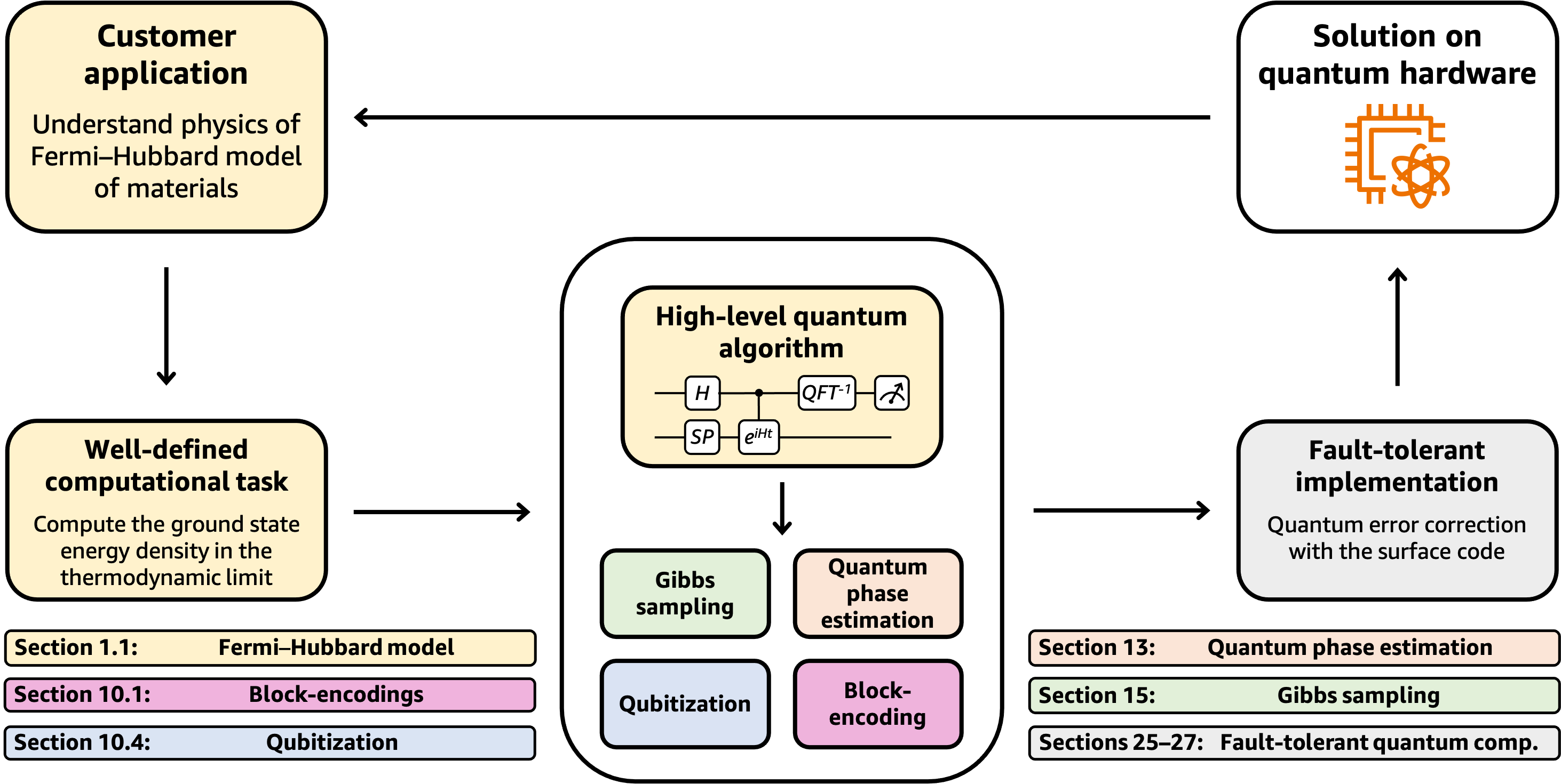
Figure 3: Example of how a fault-tolerant quantum computer could be used to accomplish the customer goal of understanding the physics of the Fermi–Hubbard model, enabling an end-to-end resource estimate. Each color corresponds to a topic covered in a certain section of the survey, noted at the bottom.

Algorithmic primitives

We have defined the computational task and outlined the high-level quantum algorithm. Now let us provide more detail on the algorithmic primitives that comprise the high-level algorithm mentioned above, and perform a full end-to-end resource estimate.

State preparation via Gibbs sampling or other methods: The complexity of preparing a good initial state is difficult to make concrete statements about, as the proposed methods are often heuristic, requiring empirical rather than analytical evaluation. In the general case, it is possible that the complexity scales exponentially in N, rendering the algorithm unusable (see, e.g., [3]). On the other hand, since systems in nature are typically found in their ground state, deep-rooted intuition from physics suggests that one should be able to prepare these states efficiently on the quantum computer by emulating nature. Toward this end, recent work by researchers at the AWS Center for Quantum Computing [4] has bolstered the theory behind Gibbs sampling, that is, the task of preparing a state in thermal equilibrium, which may be well suited to preparing good initial states for the Fermi–Hubbard model. Gibbs sampling is discussed independently in Section 15 of the survey.

Qubitization and quantum phase estimation: In the Fermi–Hubbard section of the survey (Section 1.1), the survey discusses how “quantum phase estimation” applied to a “qubitization unitary” can be used to compute the ground state energy. But how do the resource requirements of these algorithmic primitives scale, and how are they implemented? By following the embedded hyperlinks in the survey directly to the sections on quantum phase estimation (Section 13) and qubitization (Section 10.4), you can quickly determine the answers to these questions.

Specifically, the survey mentions that quantum phase estimation makes roughly α/(NΔE) calls to the qubitization unitary to compute the energy density to precision ΔE. Here, α is a normalization constant of a “block-encoding” of the Fermi–Hubbard Hamiltonian used to implement the qubitization operator. The corresponding page of the survey on block-encodings (Section 10.1) describes how they can be implemented, based on knowledge of the Hamiltonian. In particular, the “linear combinations of unitaries“ (LCU) input model is well suited due to the possible decomposition of the Fermi–Hubbard Hamiltonian as a sum of a small number of Pauli-tensor-product terms. That section also describes how to compute α in this setting, and with a small amount of calculation gives [5]

α = (2t + U/8)N

The cost of the block-encoding via LCU is given by one call to an operation called ”SELECT“ and two calls to an operation called ”PREPARE.“ While the survey does not describe optimal implementations of these operations for the Fermi–Hubbard model, SELECT has a simple (suboptimal) implementation via multi-controlled Pauli gates for the Fermi–Hubbard model, while the survey discusses methods for state preparation from classical data (used for the PREPARE operation) in Section 17.2.

The information provided in that section allows the reader to conclude that the number of logical gates needed to implement the block-encoding is

#gates for block-encoding ≈ 5N log(N)

Overall then, the cost of quantum phase estimation will be roughly

G = #gates for quantum phase estimation

≈ (2t + U/8) ⋅ 5N log(N) ⋅ (ΔE)^-1

Plugging in the value U = 8t, ΔE ≈ 10^-4t, and N = 2L² = 800, which would match the performance of classical methods in Figure 2, the calculation yields G ≈ 10⁹ gates. This can be compared to similar (but more carefully optimized) resource estimates highlighted in the survey, which obtain around 10⁸ logical gates for slightly smaller and less challenging instances [6]. Approximately Q = N + log(N) ≈ 810 logical qubits are required to run the calculation.

Fault-tolerant implementation: Next, we consider the resources needed to implement this circuit with fault tolerance. Sections 25–27 of the survey provide background information on fault tolerance. The sections explain that the surface code, depicted in Figure 4, is the most commonly-chosen quantum error-correcting code for implementation proposals due to its natural compatibility with hardware layouts and tolerance of high error rates. Additionally, Section 27 provides a worked example of a resource estimate using the surface code.

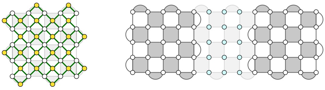
Figure 4: Fault-tolerant quantum computation with the surface code. (left) A single logical qubit is encoded into a 2D patch containing roughly 2d² physical qubits, including ancillas for error syndrome measurement, where d is the code distance. (right) Gates between two logical qubits encoded in separate patches are performed with lattice surgery. This adds additional physical qubit overhead for routing space (faded out region) and resource state distillation, incurring roughly a factor of 2.

In particular, the fault-tolerance sections present important resource formulas, which balance the exponential error suppression of the surface code against the number of faults that can arise given the number of logical qubits and gates in the algorithm. For a physical noise rate of 0.1%, the formula asserts that a distance d = 27 surface code is sufficient. In the most straightforward method for applying logical gates one after another, the number of physical qubits needed to support the computation is 4Qd² = 2.4 million, and the amount of time required is Gd𝜏, where 𝜏 is the time needed to perform a measurement of the error information (the “syndrome”), which depends on the hardware platform.

Estimated resources to perform the computation on hardware and process the outcomes: While no fault-tolerant devices currently exist, for the purpose of the resource estimate, the value of 𝜏 can be predicted based on the hardware platform. For superconducting qubits, a reasonable estimate for 𝜏 is one microsecond, leading to a total runtime estimate of 7.5 hours for the 2.4 million qubit device. As discussed above, to solve the computational task relevant to the customer, we need to repeat this calculation around 10 times, and then extrapolate to the thermodynamic limit. The calculations needed for extrapolation are smaller than the one above, hence we expect the task to be completed within a few days.

Caveats: In this example, we have ignored the failure probability of quantum phase estimation, and in our estimate, we have not accounted for the cost of ground state preparation, although these are both discussed in detail in the survey.

Summary: This example illustrates how the information presented in the survey helps to organize and streamline assessments of the feasibility of quantum algorithms for concrete customer problems. Moreover, the survey makes it straightforward to see how estimates can change if assumptions are varied. For example, try to use the survey to see how the resources are reduced if the physical error rate is instead lowered to 0.01%!

For readers interested in diving even deeper, the survey lists references where the state-of-the-art techniques for specific problems are found. For example, information about how to implement the SELECT unitary for the Fermi–Hubbard model with cost 10N logical gates is found in Ref. [6]. For ease of use and modularity, each section of the survey ends with its own reference list, and a consolidated bibliography appears at the end of the document.

Outlook and future developments

We expect the story to continue to evolve. New quantum algorithms and approaches to fault tolerance and quantum error correction are likely to be discovered, and existing ones further improved. The survey will help readers assess the context and impact of these developments in quantum technology.

On the other hand, classical computers continue to grow in scale and speed, and classical algorithms are being continually refined and developed, thereby moving the goalposts for end-to-end quantum speedups.

Quantum hardware is not yet capable of performing the fault-tolerant quantum algorithms discussed in this blog post or in the survey. While the field develops devices able to support quantum error correction, researchers and customers are exploring NISQ algorithms, which can run on hardware today, but are typically more difficult to study analytically since in most cases they are based on heuristics. With Amazon Braket, the quantum computing service of AWS, you can have on-demand access to a variety of different NISQ quantum computers to design and investigate near-term algorithms, research and develop error mitigation strategies, or run analog Hamiltonian simulations of physical spin systems and certain optimization problems. To get started, visit our webpage or explore the Amazon Braket example notebooks.

With hardware capabilities rapidly advancing, small fault-tolerant devices are now on the horizon. Scaled-up versions of these small devices will support the customer applications covered in the survey, but some applications will require many more resources than others. As we approach the age of fault-tolerant quantum computation, it is more important than ever to have a full view of the end-to-end quantum application pipeline. We hope that readers of the survey are inspired to enter this new era with the knowledge to confidently navigate this uncharted territory.

References

[1] AWS Center for Quantum Computing. “Quantum algorithms: A survey of applications and end-to-end complexities.” arXiv:2310.03011 (2023). https://arxiv.org/abs/2310.03011.

[2] LeBlanc, et al. “Solutions of the Two-Dimensional Hubbard Model: Benchmarks and Results from a Wide Range of Numerical Algorithms.“ Phys. Rev. X 5, 041041 (2015). https://doi.org/10.1103/PhysRevX.5.041041.

[3] Lee, et al. “Evaluating the evidence for exponential quantum advantage in ground-state quantum chemistry.” Nat. Commun. 14, 1952 (2023). https://doi.org/10.1038/s41467-023-37587-6.

[4] Chen, Kastoryano, Brandão, Gilyén. “Quantum Thermal State Preparation.” (2023) https://arxiv.org/abs/2303.18224.

[5] Campbell. “Early fault-tolerant simulations of the Hubbard model.” Quantum Sci. Technol. 7 015007 (2022). https://doi.org/10.1088/2058-9565/ac3110

[6] Babbush, et al. “Encoding Electronic Spectra in Quantum Circuits with Linear T Complexity.” Phys. Rev. X 8, 041015 (2018). https://doi.org/10.1103/PhysRevX.8.041015.