Monitoring SageMaker ML Models with WhyLabs

Guest post written by Danny D. Leybzon, WhyLabs MLOps Architect and Ganapathi Krishnamoorthi, AWS Solutions Architect

As the real-world changes, machine learning models degrade in their ability to accurately represent it, resulting in model performance degradation. That’s why it’s important for data scientists and machine learning engineers to support models with tools that provide ML monitoring and observability, thereby preventing that performance degradation. In this blog post, we will dive into the WhyLabs AI Observatory, a data and ML monitoring and observability platform, and show how it complements Amazon SageMaker.

Amazon SageMaker is incredibly powerful for training and deploying machine learning models at scale. WhyLabs allows you to monitor and observe your machine learning model, ensuring that it doesn’t suffer from performance degradation and continues to provide value to your business. Today, we’re going to demonstrate how to use WhyLabs to identify training-serving skew in a computer vision example for a model trained and deployed with SageMaker. WhyLabs is unique in its ability to monitor computer vision models and image data; whylogs library is able to extract features and metadata from images, as described in Detecting Semantic Drift within Image Data. The ability to create profiles based on images means that users can identify differences between training data and serving data and understand whether they need to retrain their models.

To follow along with this tutorial, we’ll utilize the WhyLabs AI Observatory, which you can access through the WhyLabs free, self-serve Starter tier.

Prepare the data and profile the training dataset with whylogs

The WhyLabs AI Observatory helps data scientists and machine learning engineers prevent model performance degradation by allowing them to monitor machine learning models, the data being fed to them, and the inferences they generate. It leverages the open-source library whylogs to generate “data profiles” (statistical summaries of datasets); these profiles are then sent to the WhyLabs platform, which allows users to analyze and alert on changes in these profiles over time.

For this example, we will build a simple model using SageMaker’s built-in algorithm for multi-label Image Classification. We will leverage whylogs’ unique ability to profile image data for data profiling and send the profiles to the WhyLabs platform for monitoring and observability. We are leveraging pycocotools 2017 images dataset for this example. This is a huge dataset with over 80 classes of images. For ease of use, we will consider only four classes and profile one image per class in the training dataset and send it to the WhyLabs platform.

The model in this blog was built using Python3 in an AWS environment on a Jupyter notebook instance. You can also run it in a Jupyter notebook on a local machine configured to run Amazon SageMaker training jobs. You will need an instance with Python3 and other Python libraries like SageMaker and WhyLabs used in the code. The dataset that we use is closer to 1GB, so make sure you have enough space in your notebook instance to download and process this dataset.

The IAM role attached to the notebook should have read and write permissions to Amazon Simple Storage Service (Amazon S3), and it should also have the access to launch training jobs and deployment endpoints in SageMaker. If you are running your notebook outside of AWS, you may want to ensure that you assume an IAM role that has these permissions attached.

Let this dissect the code to understand the flow.

First, we need to download pycocotools and install Python libraries using pip install.

import sys
!{sys.executable} -m pip install pycocotools
!pip install seaborn --upgrade
!pip install whylogs==0.6.8.dev0

Next, we will need to import certain libraries, including the SageMaker library for model training and deployment, the whylogs library for data profiling, and some standard Python libraries for numeric and image data manipulation.

import sagemaker
from sagemaker import get_execution_role
import whylogs
from whylogs import get_or_create_session
import numpy as np
from PIL import Image
import os
import json
import urllib.request
from pycocotools.coco import COCO
import datetime
import pandas as pd
from whylogs.app import Session
from whylogs.app.writers import WhyLabsWriter
 
role = get_execution_role()
print(role)
 
sess = sagemaker.Session()
bucket = sess.default_bucket()
prefix = "ic-multilabel"
 
print("using bucket %s" % bucket)

In order to utilize WhyLabs, we need to specify an API key and org ID as environment variables. To generate your own API key and org ID, follow this documentation for generating the key and ID using your free WhyLabs account.

# Set WhyLabs config variables
WHYLABS_API_KEY = "api.KEY"
WHYLABS_DEFAULT_ORG_ID = "org-12345"
 
# Set environment variables
os.environ["WHYLABS_API_KEY"] = WHYLABS_API_KEY
os.environ["WHYLABS_DEFAULT_ORG_ID"] = WHYLABS_DEFAULT_ORG_ID
 
today = datetime.datetime.now()
yesterday = today - datetime.timedelta(days=1)

We will use SageMaker’s built-in algorithm for image classification by referencing the latest container image as below

training_image = sagemaker.image_uris.retrieve(
 	region=sess.boto_region_name, framework="image-classification", version="latest"
)

Next, we’ll download the images from pycocotools. In our example, we will download a 2017 version of the image repository called ‘val2017,’ which also comes with an annotations json file.

def download(url):
 	filename = url.split("/")[-1]
 	if not os.path.exists(filename):
 	urllib.request.urlretrieve(url, filename)
 
# MSCOCO validation image files
download("http://images.cocodataset.org/zips/val2017.zip")
download("http://images.cocodataset.org/annotations/annotations_trainval2017.zip")

As a standard practice, we will unzip the file to access the underlying images and annotations file.

!unzip -qo val2017.zip
!unzip -qo annotations_trainval2017.zip

To make it simple, we will choose the first four classes in pycocotools images for extraction. The category ids are mapped as below:

1. Person
2. Bicycle
3. Car
4. Motorcycle

We will use pycocotools built-in libraries to extract images from these four classes by referring to the annotations and creating a lst file. A lst file is a text file that consists of a list of pointers to images in other files. The below code snippet gets the four image categories listed above and extracts the images within each category. A lst file is constructed with the image ids and the labels as shown below.

annFile = "./annotations/instances_val2017.json"
coco = COCO(annFile)
catIds = coco.getCatIds()
 
image_ids_of_cats = []
 
for cat in catIds:
 	image_ids_of_cats.append(coco.getImgIds(catIds=cat))
 
image_ids = []
labels = []
# use only the first 4 classes
# obtain image ids and labels for images with these 4 classes
 
cats = [1,2,3,4]
 
for ind_cat in cats:
 	for image_id in image_ids_of_cats[ind_cat - 1]:
 	if image_id in image_ids:
       	labels[image_ids.index(image_id)][ind_cat - 1] = 1
 	else:
       	image_ids.append(image_id)
       	labels.append(np.zeros(len(cats), dtype=np.int))
       	labels[-1][ind_cat - 1] = 1
       	 
# Construct the lst file from the image ids and labels
# The first column is the image index, the last is the image filename
# and the second to last but one are the labels
with open("image.lst", "w") as fp:
 	sum_labels = labels[0]
    
 	for ind, image_id in enumerate(image_ids):
 	coco_img = coco.loadImgs(image_id)
 	image_path = os.path.join(coco_img[0]["file_name"])
 	label_h = labels[ind]
 	sum_labels += label_h
 	fp.write(str(ind) + "\t")
 	for j in label_h:
       	fp.write(str(j) + "\t")
 	fp.write(image_path)
 	fp.write("\n")
       	 
 	fp.close()
print(sum_labels)

Now that we’ve extracted our training data, we can profile it and send those profiles to WhyLabs in a few easy lines of code.

writer = WhyLabsWriter("", formats=[],)
session = Session(project="demo-project", pipeline="pipeline-id", writers=[writer])
with session.logger(tags={"datasetId": "model-1"},dataset_timestamp = yesterday) as ylog:
 	# Profiling a sample image for person
 	ylog.log_image("val2017/000000066231.jpg")
 	# Profiling a sample image for bicycle
 	ylog.log_image("val2017/000000169996.jpg")
 	# Profiling a sample image for car
 	ylog.log_image("val2017/000000204871.jpg")
 	# Profiling a sample image for motorcycle
 	ylog.log_image("val2017/000000136715.jpg")

Profiling these images should take less than a second. From here, we can navigate back to the WhyLabs UI (where we had previously generated our API key) and head to the Model Dashboard to verify that our model is now populated with these profiles.

As we can see, our “Image Classifier” model is now populated with some profiles. We can explore this “baseline” training profile by navigating to the model summary page and then drilling down to that particular profile.

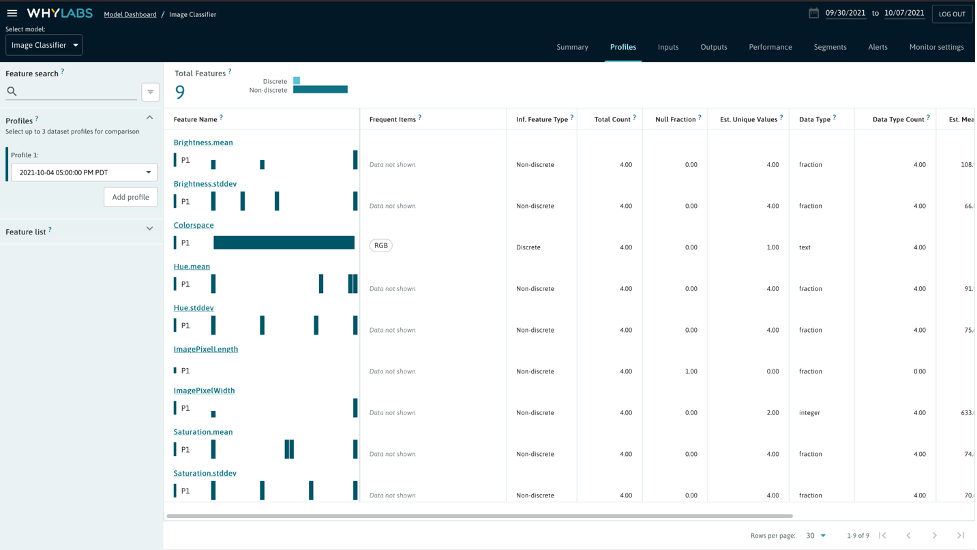
As illustrated above, whylogs was able to extract some key metadata (such as the pixel width and pixel height) and image features (such as the brightness mean and the standard deviation within the saturation) from the images we fed it. One particularly interesting piece of metadata is the ImagePixelWidth, which we will return to after uploading a profile from our inference dataset that doesn’t match the training dataset.

Train and deploy the model with Amazon SageMaker

Let us now move on to our standard practice of creating the lst file and splitting the input dataset into train and validation channels for the image file and the lst file.

!shuf image.lst > im.lst
!head -n 2500 im.lst > mscocoval2017train.lst
!tail -n +2501 im.lst > mscocoval2017val.lst
!head mscocoval2017train.lst
!wc -l mscocoval2017train.lst
!wc -l mscocoval2017val.lst
 
# Four channels: train, validation, train_lst, and validation_lst
s3train = "s3://{}/{}/train/".format(bucket, prefix)
s3validation = "s3://{}/{}/validation/".format(bucket, prefix)
s3train_lst = "s3://{}/{}/train_lst/".format(bucket, prefix)
s3validation_lst = "s3://{}/{}/validation_lst/".format(bucket, prefix)
 
# upload the image files to train and validation channels
!aws s3 cp val2017 $s3train --recursive --quiet
!aws s3 cp val2017 $s3validation --recursive --quiet
 
# upload the lst files to train_lst and validation_lst channels
!aws s3 cp mscocoval2017train.lst $s3train_lst --quiet
!aws s3 cp mscocoval2017val.lst $s3validation_lst --quiet

We now configure the SageMaker training job with required parameters including the container image for object detection algorithm, IAM role, type of training instances, number of training instances, maximum training time in seconds, EBS volume storage, input mode and output location of the model artifact. For deep learning, we normally recommend GPU instance families like P2, P3 etc. as training is much faster on a GPU instance, but if you are on a budget or attempting to explore and learn, you can use CPU instances like C5, C4 and C3. In the below code we are using a GPU instance for training.

s3_output_location = "s3://{}/{}/output".format(bucket, prefix)
multilabel_ic = sagemaker.estimator.Estimator(
 	training_image,
 	role,
 	instance_count=1,
 	instance_type="ml.p2.xlarge",
 	volume_size=50,
 	max_run=360000,
 	input_mode="File",
 	output_path=s3_output_location,
 	sagemaker_session=sess,
)

With any SageMaker training, it’s important to set hyperparameters for better accuracy. Every built-in algorithm would need a certain set of hyperparameters (required and optional) to be tuned as listed in the documentation. Here we set some static values to hyperparameters, but you can also pass on a range of values in a json document as shown here.

multilabel_ic.set_hyperparameters(
 	num_layers=18,
 	use_pretrained_model=1,
 	image_shape="3,224,224",
 	num_classes=5,
 	mini_batch_size=128,
 	resize=256,
 	epochs=5,
 	learning_rate=0.001,
 	num_training_samples=2500,
 	use_weighted_loss=1,
 	augmentation_type="crop_color_transform",
 	precision_dtype="float32",
 	multi_label=1,
)

We then set up four different channels for the SageMaker training job as below and kick off a training job.

train_data = sagemaker.inputs.TrainingInput(
 	s3train,
 	distribution="FullyReplicated",
 	content_type="application/x-image",
 	s3_data_type="S3Prefix",
)
validation_data = sagemaker.inputs.TrainingInput(
 	s3validation,
 	distribution="FullyReplicated",
 	content_type="application/x-image",
 	s3_data_type="S3Prefix",
)
train_data_lst = sagemaker.inputs.TrainingInput(
 	s3train_lst,
 	distribution="FullyReplicated",
 	content_type="application/x-image",
 	s3_data_type="S3Prefix",
)
validation_data_lst = sagemaker.inputs.TrainingInput(
 	s3validation_lst,
 	distribution="FullyReplicated",
 	content_type="application/x-image",
 	s3_data_type="S3Prefix",
)
data_channels = {
 	"train": train_data,
 	"validation": validation_data,
 	"train_lst": train_data_lst,
 	"validation_lst": validation_data_lst,
}

We now kick off the SageMaker training job that we just configured with a fit command.

multilabel_ic.fit(inputs=data_channels, logs=True)

Once the training completes, we deploy the model to a real-time SageMaker endpoint, so we can start inferencing. With this deployment, SageMaker spins up server(s) for inference based on the configuration, deploys the model artifact and processes inference payloads. We go on to configure instance type, instance count and serializer library for the SageMaker deployment endpoint as shown below. You can also refer to the recommended instance types for built-in algorithms here.

from sagemaker.serializers import IdentitySerializer
 
ic_classifier = multilabel_ic.deploy(
 	initial_instance_count=1,
 	instance_type="ml.m4.xlarge",
 	serializer=IdentitySerializer(content_type="application/x-image"),
)

The model is now ready for inference.

Make a prediction on out-of-distribution data

We will now showcase how WhyLabs can be effective in this scenario by taking an image from a class outside of what the model was trained on and lowering the image resolution. This realistically represents training-serving skew, where the data used to build the model is different from the data that the model tries to infer against in production. We can then use WhyLabs to analyze the inference data and see how it differs from the training data.

Let’s pick an image from a different class outside of what the model was trained and lower the image resolution.

## Profiling bird image
img = Image.open('val2017/000000147498.jpg')
print(img.size)
 
red_res_image = img.resize((200, 120))
red_res_image.save('low_res_image.jpg')

Now, let’s generate a whylogs profile of that image and send it to WhyLabs.

writer = WhyLabsWriter("", formats=[],)
session = Session(project="demo-project", pipeline="pipeline-id", writers=[writer])
with session.logger(tags={"datasetId": "model-1"},dataset_timestamp = today) as ylog:
 	# Profiling the inference image with reduced resolution
 	ylog.log_image("low_res_image.jpg")

In the WhyLabs UI, we can now see that we have two profiles for this model: one for training and one for inference:

We can see that our new profile has the same features as the old one:

And compare the two:

Looking at the ImagePixelWidth feature specifically, we can observe that the width of the images in first profile is significantly higher than in the second profile, indicating that our inference data is lower in resolution.

In this exercise, we’ve used a very simple example, and we knew that there would be some disparity (training-serving skew) because we set the training and inference data to be different. In the real world, this would be a clear indicator that our model might not perform as well in production as it did during our initial testing in our training sandbox. As an action to such an indication, we might need to take into account that lower image resolution leads to lower model accuracy and potentially retrain our model to help mitigate that.

Conclusion

Following the steps above, we trained a computer vision model in SageMaker and monitored the input image data with WhyLabs. We intentionally created synthetic data for production that didn’t match the data being used for training the model, so that we could highlight WhyLabs’ ability to identify training-serving skew. In the real world, data scientists don’t intentionally make their production data mismatch their training data. However, data in the real world tend to be messier and more prone to produce errors than those used by data scientists during the training and validation phase.

Training-service skew is one of a number of different examples of problems that can cause model performance degradation in production environments, but through this example, we saw how WhyLabs can help reduce this risk in image data. For those working with other formats, text support is available now, and video and speech data support will be coming soon.

To get support for the open source whylogs library, the self-serve AI Observatory, or for any ML monitoring questions, join the WhyLabs Community Slack.

	Danny D. Leybzon is an MLOps Architect at WhyLabs. Danny evangelizes machine learning best practices and has helped countless customers bring their ML models out of the sandbox and into production. When Danny isn’t thinking, talking, or writing about MLOps, he’s hiking, skiing, or scuba diving.
	Ganapathi Krishnamoorthi is a Senior Solutions Architect at AWS. Ganapathi provides prescriptive guidance to enterprise customers helping them to design and deploy cloud applications at scale. He is passionate about machine learning and is focused on helping customers leverage AI/ML for their business outcomes. When not at work, he enjoys exploring outdoors and listening to music.