Exploratory data analysis of genomic datasets using ADAM and Mango with Apache Spark on Amazon EMR

As the cost of genomic sequencing has rapidly decreased, the amount of publicly available genomic data has soared over the past couple years. New cohorts and studies have produced massive datasets consisting of over 100,000 individuals. Simultaneously, these datasets have been processed to extract genetic variation across populations, producing mass amounts of variation data for each cohort. In this era of big data, tools like Apache Spark have provided a user-friendly platform for batch processing large datasets. However, in order to use such tools as a sufficient replacement to current bioinformatics pipelines, we need more accessible and comprehensive API’s for processing genomic data, as well as support for interactive exploration of these processed datasets.

ADAM and Mango provide a unified environment for processing, filtering, and visualizing large genomic datasets on Apache Spark. ADAM allows users to programmatically load, process, and select raw genomic and variation data using SparkSQL, an SQL interface for aggregating and selecting data in Apache Spark. Mango supports visualization of both raw and aggregated genomic data in a Jupyter notebook environment, allowing users to draw conclusions from large datasets at multiple resolutions. This combined power of ADAM and Mango allows users to load, query and explore datasets in a unified environment, allowing users to interactively explore genomic data at a scale previously impossible using single node bioinformatics tools.

Configuring ADAM and Mango on Amazon EMR

First, we will launch and configure an EMR cluster. Mango uses Docker containers to easily run on Amazon EMR. Upon cluster startup, EMR will use the bootstrap action below to install Docker and the required startup scripts. The scripts will be available at /home/hadoop/mango-scripts

aws emr create-cluster 
--release-label emr-5.19.0 \   
--name 'emr-5.19.0 Mango example' \   
--applications Name=Hadoop Name=Hive Name=Spark \   
--ec2-attributes KeyName=<your-ec2-key>,InstanceProfile=EMR_EC2_DefaultRole \   
--service-role EMR_DefaultRole \     
--instance-groups \     InstanceGroupType=MASTER,InstanceCount=1,InstanceType=c5.4xlarge \     InstanceGroupType=CORE,InstanceCount=4,InstanceType=c5.4xlarge \   --region <your-aws-region> \   
--log-uri s3://<your-s3-bucket>/emr-logs/ \   
--bootstrap-actions \     
Name='Install Mango', Path="s3://aws-bigdata-blog/artifacts/mango-emr/install-bdg-mango-docker-emr5.sh"

To start the Mango notebook, run the following:

/home/hadoop/mango-scripts/run-notebook.sh

This file will set up all of the environment variables needed to run Mango in Docker on EMR. In your terminal, you will see the port and Jupyter notebook token for the Mango Notebook session. Navigate to this port on the public DNS URL of the master node for your EMR cluster.

Loading data from the 1000 Genomes Project

Now that we have a working environment, lets use ADAM and Mango to discover interesting variants in the child from the genome sequencing data of a trio (data from a mother, father, and child). These data are available from the 1000 Genomes Project AWS Public Dataset. In this analysis, we will view a trio (NA19685, NA19661, and NA19660) and search for variants that are present in the child but not present in the parents.

In particular, we want to identify genetic variants that are found in the child but not in the parents, known as de novo variants. These are interesting regions, as they may indicate sights of de novo variation that may contribute to multiple disorders.

You can find the Jupyter notebook containing these examples in Mango’s GitHub repository, or at /opt/cgl-docker-lib/mango/example-files/notebooks/aws-1000genomes.ipynb in the running Docker container for Mango.

First, import the ADAM and Mango modules and any Spark modules that you need:

# Import ADAM modules
from bdgenomics.adam.adamContext import ADAMContext
from bdgenomics.adam.rdd import AlignmentRecordRDD, CoverageRDD
from bdgenomics.adam.stringency import LENIENT, _toJava

# Import Mango modules
from bdgenomics.mango.rdd import GenomicVizRDD
from bdgenomics.mango.QC import CoverageDistribution

# Import Spark modules
from pyspark.sql import functions as sf

Next, create a Spark session. You will use this session to run SQL queries on variants.

# Create ADAM Context
ac = ADAMContext(spark)

Variant analysis with Spark SQL

Load in a subset of variant data from chromosome 17:

genotypesPath = 's3://1000genomes/phase1/analysis_results/integrated_call_sets/ALL.chr17.integrated_phase1_v3.20101123.snps_indels_svs.genotypes.vcf.gz'
genotypes = ac.loadGenotypes(genotypesPath)

# repartition genotypes to balance the load across memory
genotypes_df  = genotypes.toDF()

You can take a look at the schema by printing the columns in the dataframe.

# cache genotypes and show the schema
genotypes_df.columns

This genotypes dataset contains all samples from the 1000 Genomes Project. Therefore, you will next filter genotypes to only consider samples that are in the NA19685 trio, and cache the results in memory.

# trio IDs
IDs = ['NA19685', 'NA19661','NA19660']

# Filter by individuals in the trio
trio_df = genotypes_df.filter(genotypes_df["sampleId"].isin(IDs))

trio_df.cache()
trio_df.count()

Next, add a new column to your dataframe that determines the genomic location of each variant. This is defined by the chromosome (contigName) and the start and end position of the variant.

# Add ReferenceRegion column and group by referenceRegion
trios_with_referenceRegion = trio_df.withColumn('ReferenceRegion', 
                    sf.concat(sf.col('contigName'),sf.lit(':'), sf.col('start'), sf.lit('-'), sf.col('end')))

Now, you can query your dataset to find de novo variants. But first, you must register your dataframe with Spark SQL.

#  Register df with Spark SQL
trios_with_referenceRegion.createOrReplaceTempView("trios")

Now that your dataframe is registered, you can run SQL queries on it. For the first query, select the names of variants belonging to sample NA19685 that have at least one alternative (ALT) allele.

# filter by alleles. This is a list of variant names that have an alternate allele for the child
alternate_variant_sites = spark.sql("SELECT variant.names[0] AS snp FROM trios \
                                    WHERE array_contains(alleles, 'ALT') AND sampleId == 'NA19685'") 

collected_sites = list(map(lambda x: x.snp, alternate_variant_sites.collect())

For your next query, filter sites in which the parents have both reference alleles. Then filter these variants by the set produced previously from the child.

# get parent records and filter by only REF locations for variant names that were found in the child with an ALT
filtered1 = spark.sql("SELECT * FROM trios WHERE sampleId == 'NA19661' or sampleId == 'NA19660' \
            AND !array_contains(alleles, 'ALT')")
filtered2 = filtered1.filter(filtered1["variant.names"][0].isin(collected_sites))
snp_counts = filtered2.groupBy("variant.names").count().collect()

# collect snp names as a list
snp_names = map(lambda x: x.names, snp_counts)
denovo_snps = [item for sublist in snp_names for item in sublist]
denovo_snps[:10]

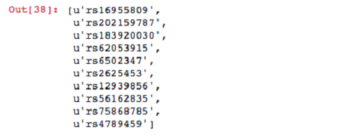
Now that you have found some interesting variants, you can unpersist your genotypes from memory.

trio_df.unpersist()

Working with alignment data

You have found a lot of potential de novo variant sites. Next, you can visually verify some of these sites to see if the raw alignments match up with these de novo hits.

First, load in the alignment data for the NA19685 trio:

# load in NA19685 exome from s3a

childReadsPath = 's3a://1000genomes/phase1/data/NA19685/exome_alignment/NA19685.mapped.illumina.mosaik.MXL.exome.20110411.bam'
parent1ReadsPath = 's3a://1000genomes/phase1/data/NA19685/exome_alignment/NA19660.mapped.illumina.mosaik.MXL.exome.20110411.bam'
parent2ReadsPath = 's3a://1000genomes/phase1/data/NA19685/exome_alignment/NA19661.mapped.illumina.mosaik.MXL.exome.20110411.bam'

childReads = ac.loadAlignments(childReadsPath, stringency=LENIENT)
parent1Reads = ac.loadAlignments(parent1ReadsPath, stringency=LENIENT)
parent2Reads = ac.loadAlignments(parent2ReadsPath, stringency=LENIENT)

Note that this example uses s3a:// instead of s3:// style URLs. The reason for this is that the ADAM formats use Java NIO to access BAM files. To do this, we are using a JSR 203 implementation for the Hadoop Distributed File System to access these files. This itself requires the s3a:// protocol. You can view that implementation in this GitHub repository.

You now have data alignment data for three individuals in your trio. However, the data has not yet been loaded into memory. To cache these datasets for fast subsequent access to the data, run the cache() function:

# cache child RDD and count records
# takes about 2 minutes, on 4 c3.4xlarge worker nodes 
childReads.cache()

# Count reads in the child
childReads.toDF().count()
# Output should be 95634679

Quality control of alignment data

One popular analysis to visually re-affirm the quality of genomic alignment data is by viewing coverage distribution. Coverage distribution gives you an idea of the read coverage that you have across a sample.

Next, generate a sample coverage distribution plot for the child alignment data on chromosome 17:

# Calculate read coverage
# Takes 2-3 minutes
childCoverage = childReads.transform(lambda x: x.filter(x.contigName == "17")).toCoverage()

childCoverage.cache()
childCoverage.toDF().count()

# Output should be 51252612

Now that coverage data is calculated and cached, compute the coverage distribution of chromosome 17 and plot the coverage distribution:

# Calculate coverage distribution

# You can check the progress in the SparkUI by navigating to 
# :8088 and clicking on the currently running Spark application.
cd = CoverageDistribution(spark, childCoverage, bin_size = 1)
ax, results = cd.plotDistributions(normalize=True, cumulative=False)

ax.set_title("Normalized Target Region Coverage")
ax.set_ylabel("Fraction")
ax.set_xlabel("Coverage Depth")
ax.set_xscale("log")
plt.show()

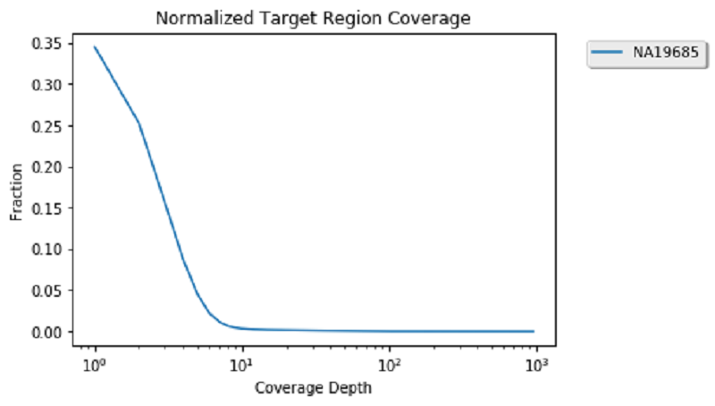
This looks pretty standard because the data you are viewing is exome data. Therefore, you can see a high number of sights with low coverage and a smaller number of genomic positions with more than 100 reads. Now that you are done with coverage, you can unpersist these datasets to clear space in memory for the next analysis.

childCoverage.unpersist()

Viewing sites with missense variants in the proband

After verifying alignment data and filtering variants, you have four genes with potential missense mutations in the proband, including YBX2, ZNF286B, KSR1, and GNA13. You can visually verify these sites by filtering and viewing the raw reads of the child and parents.

First, view the child reads. If you zoom in to the location of the GNA13 variant (63052580-63052581), you can see a heterozygous T to A call:

# missense variant at GNA13: 63052580-63052581 (SNP rs201316886)
# define alignment summary for child reads
childViz = AlignmentSummary(spark, ac, childReads)

# Takes about 2 minutes to collect data from workers
contig = "17"
start = 63052180
end = 63052981

childViz.viewPileup(contig, start, end)

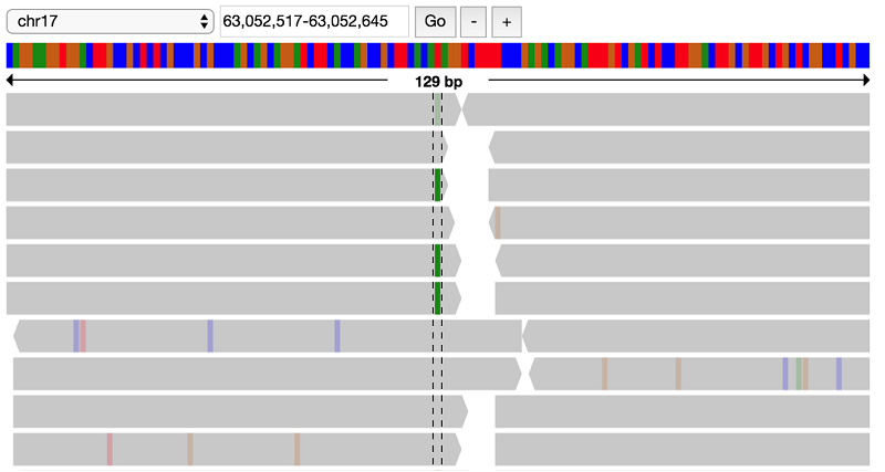
It looks like there indeed is a variant at this position, possibly a heterozygous SNP with alternate allele A. Look at the parent data to verify that this variant does not appear in the parents:

# define alignment summary for parent reads
parent1Viz = AlignmentSummary(spark, ac, parent1Reads)

# view missense variant at GNA13: 63052580-63052581 in parent 1
contig = "17"
start = 63052180
end = 63052981

parent1Viz.viewPileup(contig, start, end)

This confirms the filter that this variant is indeed present only in the proband, but not the parents.

Summary

To summarize, this post demonstrated how to set up and run ADAM and Mango in Amazon EMR. We demonstrated how to use these tools in an interactive notebook environment to explore the 1000 Genomes dataset, a publicly available dataset on Amazon S3. We used these tools inspect 1000 Genomes data quality, query for interesting variants in the genome, and validate results through the visualization of raw data.

For more information about Mango, see the Mango User Guide. If you have questions or suggestions, please comment below.

Additional Reading

If you found this post useful, be sure to check out Genomic Analysis with Hail on Amazon EMR and Amazon Athena, Interactive Analysis of Genomic Datasets Using Amazon Athena, and, on the AWS Compute Blog, Building High-Throughput Genomics Batch Workflows on AWS: Introduction (Part 1 of 4).

About the Author

Alyssa Marrow is a graduate student in the RISELab and Yosef Lab at the University of California Berkeley. Her research interests lie at the intersection of systems and computational biology. This involves building scalable systems and easily parallelized algorithms to process and compute on all that ‘omics data.