Demand intelligence made simple with PredictHQ event data through AWS Data Exchange and Amazon SageMaker

No matter your business, events likely have a major impact on your demand. Using various solutions from Amazon Web Services (AWS), companies can gain access to high-quality and enriched event data that helps them analyze what’s happening in the real world at a massive scale. This in turn can help them make decisions around staffing, inventory, pricing, site selection, on-time delivery, and more.

Event data can be consumed in a variety of ways, including through PredictHQ’s various APIs, as well as through AWS Data Exchange, where you can find, subscribe to, and use third-party data in the cloud. This synergy between PredictHQ and AWS helps companies access intelligent event data instantaneously so that the data is always up to date, which is crucial given the dynamic nature of events.

That being said, third-party data can be complex to bring into your data warehouse or existing models. The goal of this blog is to show you, through an example, how to retrieve and integrate event features into a forecasting model running on Amazon SageMaker, an AWS cloud machine learning (ML) platform.

Overview

We’ll use real-world demand data from a restaurant customer to show you how integrating event features into an existing forecasting model can improve forecasting accuracy (root mean square error [RMSE]) by up to 20 percent or even beyond. Improved demand forecasts for restaurants have downstream impact on labor optimization, ordering, and more.

In addition to Amazon SageMaker, we’ll use an Extreme Gradient Boosting (XGBoost) model, a supervised learning algorithm used for regression and classification on large datasets.

Although we’re using Amazon SageMaker and XGBoost here, the model architecture (depicted below) used in this demo is agnostic to ML platforms and forecasting models.

Figure 1: Model architecture

Set up

Please follow this guideline to launch Amazon SageMaker Studio from the console.

Once the Amazon SageMaker studio is ready, you can clone the GitHub repository containing the Jupyter Notebook used in this blog.

Figure 2: Within Amazon SageMaker Studio, clone the Git repository containing demo artifacts

After cloning the repository, open notebook rundemo_rd_sdk.ipynb to get started.

Figure 3: Open notebook “rundemo_rd_sdk.ipynb”

Get started

After you are ready to start, the first step is to install all required Python packages to run this demo.

!pip --disable-pip-version-check install pandas
!pip --disable-pip-version-check install numpy
!pip --disable-pip-version-check install xgboost
!pip --disable-pip-version-check install predicthq


from datetime import datetime, date, timedelta

import matplotlib.pyplot as plt
import pandas as pd
import plotly.graph_objects as go
import requests
from predicthq import Client
from sklearn.metrics import mean_squared_error
from xgboost import XGBRegressor, plot_importance

In this example, we will predict the order count for a fast-casual restaurant located in Iowa City, Iowa. We have one year of historical data, dated back from 2021-06-01 to 2022-07-04. We will use 2021-06-01 to 2022-06-19 as training data, and we will predict the demand for the dates from 2022-06-20 to 2022-07-04.

We’ll use a radius of 1.76 km (1.1 miles) to search for the events near this store. This radius is a result of our suggested radius API. There are 23 venues close to this store within a 1.76 km radius.

We’ll use PredictHQ Beam to determine the event categories to focus on. Beam is the PredictHQ automated correlation engine that consists of two different models: the decomposition model and a category importance model. Beam decomposes the demand data and more to identify the statistical correlation between event categories and the demand data we’re working with, which, in this case, is the number of orders.

By running these models, we learn there are eight event categories statistically correlated to the demand:

Sports
Public holidays
School holidays
Expos
Observances
Severe weather
Concerts
Performing arts

The PredictHQ data science team can help you run your demand data through the category importance model and get access to the suggested radius API as well as decompose your data.

Get relevant event features through the Features API and process

After we’ve determined our focus event categories, we will find relevant features to use through PredictHQ Features API, which are forecast-ready prebuilt intelligence and features.

The ACCESS_TOKEN is used for preparing event features from Features API. The provided ACCESS_TOKEN is limited to the demo example. For event features in other locations or time periods, the following link will guide you through creating an account and creating an access token:

https://docs.predicthq.com/guides/quickstart/

ACCESS_TOKEN = "z8vSasLdbCFVQlymo4Ng1OPz4GoRLRo3QtpJNRhE"

DATE_FORMAT = "%Y-%m-%d"
FEATURES_API_URL = "https://api.predicthq.com/v1/features"

phq = Client(access_token=ACCESS_TOKEN)

def get_date_groups(start, end):
    """
    Features API allows a range of up to 90 days, so we have to do several requests
    """

    def _split_dates(s, e):
        capacity = timedelta(days=90)
        interval = 1 + int((e - s) / capacity)
        for i in range(interval):
            yield s + capacity * i
        yield e

    dates = list(_split_dates(start, end))
    for i, (d1, d2) in enumerate(zip(dates, dates[1:])):
        if d2 != dates[-1]:
            d2 -= timedelta(days=1)
        yield d1.strftime(DATE_FORMAT), d2.strftime(DATE_FORMAT)

First, you’ll prepare the features for attendance-based events and holiday events.

ATTENDED_FEATURES = [
    "phq_attendance_community",
    "phq_attendance_concerts",
    "phq_attendance_conferences",
    "phq_attendance_expos",
    "phq_attendance_festivals",
    "phq_attendance_performing_arts",
    "phq_attendance_sports",
]
HOLIDAY_FEATURES = [
    "phq_rank_observances",
    "phq_rank_public_holidays",
]


def get_features_api_data(lat, lon, start, end, radius=500, rank_threshold=30):
    start = datetime.strptime(start, DATE_FORMAT).date()
    end = datetime.strptime(end, DATE_FORMAT).date()

    result = []
    for gte, lte in get_date_groups(start, end):
        query = {
            "active__gte": gte,
            "active__lte": lte,
            "location__geo": {"lat": lat, "lon": lon, "radius": f"{radius}m"},
        }

        query.update({f"{f}__stats": ["sum"] for f in ATTENDED_FEATURES})
        query.update(
            {f"{f}__phq_rank": {"gte": rank_threshold} for f in ATTENDED_FEATURES}
        )
        query.update({f"{f}": True for f in HOLIDAY_FEATURES})

        features = phq.features.obtain_features(**query)

        for feature in features:
            record = {}
            for k, v in feature.to_dict().items():
                if k == "date":
                    record[k] = v.strftime("%Y-%m-%d")
                elif k in ATTENDED_FEATURES:
                    record[k] = v.get("stats", {}).get("sum")
                elif k in HOLIDAY_FEATURES:
                    record[k] = sum(float(x) for x in v.get("rank_levels", {}).values())

            result.append(record)

    return result


res = get_features_api_data(41.657871, -91.534637, "2021-06-01", "2022-07-04", 1760, 30)
df_attended_holidays = pd.DataFrame(res)

columns_constant = [
    col
    for col in df_attended_holidays.columns[1:]
    if col.replace("phq_attendance_", "").replace("phq_rank_", "")
    not in category_important_results
]
df_attended_holidays.drop(columns=columns_constant, inplace=True)
#df_attended_holidays.head(20)

Next, we’ll prepare features for school holidays.

ATTENDED_FEATURES = [
    "phq_attendance_school_holidays",
]


def get_features_api_school_holidays(lat, lon, start, end, rank_threshold=30):
    start = datetime.strptime(start, DATE_FORMAT).date()
    end = datetime.strptime(end, DATE_FORMAT).date()

    result = []
    for gte, lte in get_date_groups(start, end):
        query = {
            "active__gte": gte,
            "active__lte": lte,
            "location__geo": {"lat": lat, "lon": lon, "radius": "1m"},
        }

        query.update({f"{f}__stats": ["sum"] for f in ATTENDED_FEATURES})
        query.update(
            {f"{f}__phq_rank": {"gte": rank_threshold} for f in ATTENDED_FEATURES}
        )

        features = phq.features.obtain_features(**query)

        for feature in features:
            record = {}
            for k, v in feature.to_dict().items():
                if k == "date":
                    record[k] = v.strftime("%Y-%m-%d")
                elif k in ATTENDED_FEATURES:
                    record[k] = v.get("stats", {}).get("sum")

            result.append(record)

    return result


res = get_features_api_school_holidays(
    41.657871, -91.534637, "2021-06-01", "2022-07-04", 30
)
df_school_holidays = pd.DataFrame(res)

Finally, you’ll prepare features for severe weather events. Severe weather warnings and alerts might lead to disruption and can have a huge influence on demand.

SEVERE_WEATHER_FEATURES = {
    "phq_impact_severe_weather_air_quality_retail",
    "phq_impact_severe_weather_blizzard_retail",
    "phq_impact_severe_weather_cold_wave_retail",
    "phq_impact_severe_weather_cold_wave_snow_retail",
    "phq_impact_severe_weather_cold_wave_storm_retail",
    "phq_impact_severe_weather_dust_retail",
    "phq_impact_severe_weather_dust_storm_retail",
    "phq_impact_severe_weather_flood_retail",
    "phq_impact_severe_weather_heat_wave_retail",
    "phq_impact_severe_weather_hurricane_retail",
    "phq_impact_severe_weather_thunderstorm_retail",
    "phq_impact_severe_weather_tornado_retail",
    "phq_impact_severe_weather_tropical_storm_retail",
}


def get_features_api_severe_weather_events(lat, lon, start, end, rank_threshold=30):
    start = datetime.strptime(start, DATE_FORMAT).date()
    end = datetime.strptime(end, DATE_FORMAT).date()

    result = []
    for gte, lte in get_date_groups(start, end):
        query = {
            "active__gte": gte,
            "active__lte": lte,
            "location__geo": {"lat": lat, "lon": lon, "radius": "1m"},
        }

        query.update({f"{f}__stats": ["max"] for f in SEVERE_WEATHER_FEATURES})
        query.update(
            {f"{f}__phq_rank": {"gte": rank_threshold} for f in SEVERE_WEATHER_FEATURES}
        )

        features = phq.features.obtain_features(**query)

        for feature in features:
            record = {}
            for k, v in feature.to_dict().items():
                if k == "date":
                    record[k] = v.strftime("%Y-%m-%d")
                else:
                    record[k] = v.get("stats", {}).get("max")

            result.append(record)

    return result



res = get_features_api_severe_weather_events(
    41.657871, -91.534637, "2021-06-01", "2022-07-04", 60
)
df_severe_weather_features = pd.DataFrame(res)

columns_constant = [
    col
    for col in df_severe_weather_features.sum()[1:].to_dict().keys()
    if df_severe_weather_features[col].sum() == 0
]
df_severe_weather_features.drop(columns=columns_constant, inplace=True)
#df_severe_weather_features.head(20)

Capture severe weather events with Forecast-Ready Demand Impact Patterns and Polygons

These events impact demand before and after they occur. PredictHQ Forecast-Ready Demand Impact Patterns accurately capture the leading, lagging, and coincident effects of a severe weather event on demand.

Of course, severe weather events don’t happen at only a single location. PredictHQ Polygons help you see the full area impacted by an event represented as a shape—giving you a much more accurate picture of impact. Polygons automatically update as severe weather events change direction, severity, and area of impact. Polygons are driven by the most up-to-date, accurate weather data available—so restaurants can quickly take action.

By using Features API, you can easily get access to severe weather event features for your forecasts. Given this is one of the categories that was correlated to the number of orders for the restaurant we’re working on, we’ll use these features.

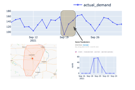
Figure 4: Polygon for severe weather events

Now that you have the features you’ll be working with, the next step is to load the demand through a comma-separated values (CSV) file and combine event features with time trend features.

# Load demand dataset
df_demand = pd.read_csv("data/demand.csv")
df_demand["date"] = pd.to_datetime(df_demand["date"])

# Convert date to time relevant feature
df_event_features["date"] = pd.to_datetime(df_event_features["date"])
df_event_features[["day_of_week", "week_of_year", "month_of_year"]] = (
    df_event_features["date"]
    .map(lambda x: [x.day_of_week, x.weekofyear, x.month])
    .to_list()
)
df = df_demand.merge(df_event_features, how="left", on="date")

Build a forecasting model with XGBoost

Now you are ready to build a forecast using the XGBoost model based on all the features.

split_date_test = "2022-06-20"
feature_columns = df.columns[2:]
demand_column = "demand"

X_train = df[df["date"] < split_date_test][feature_columns]
X_test = df[df["date"] >= split_date_test][feature_columns]
y_train = df[df["date"] < split_date_test][demand_column]
y_test = df[df["date"] >= split_date_test][demand_column]

# len(X_train), len(X_test), len(y_train), len(y_test)
feature_columns

xgb_model = XGBRegressor(
    n_estimators=100,
    learning_rate=0.1,
    max_depth=6,
    random_state=42,
    n_jobs=-1,
)
xgb_model.fit(
    X_train,
    y_train,
    verbose=True,
)
# xgb_model.save_model(f"xgb_demand_forecasting.json") #

xgb_model.predict(X_test)

Forecast the next two weeks’ demand starting from 2022-06-20.

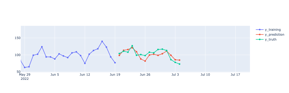
Figure 5: Forecasted demand versus actual demand

Compare forecasts with and without event features

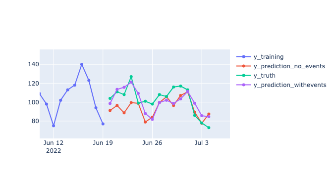
Figure 6: Compare forecast performance with and without event features

from sklearn.metrics import mean_absolute_error, mean_squared_error

MAE_model_withevents = mean_absolute_error(y_test, xgb_model.predict(X_test))
MAE_model_no_events = mean_absolute_error(
    y_test_withoutevents, xgb_model_withoutevents.predict(X_test_withoutevents)
)
MAE_Model_improvement = (
    (MAE_model_no_events - MAE_model_withevents) / MAE_model_no_events * 100
)

RMSE_model_withevents = mean_squared_error(
    y_test, xgb_model.predict(X_test), squared=False
)
RMSE_model_no_events = mean_squared_error(
    y_test_withoutevents,
    xgb_model_withoutevents.predict(X_test_withoutevents),
    squared=False,
)
RMSE_Model_improvement = (
    (RMSE_model_no_events - RMSE_model_withevents) / RMSE_model_no_events * 100
)

print(f"With event features in the model, MAE is {MAE_model_withevents:.2f}")
print(f"Without event features in the model, MAE is {MAE_model_no_events:.2f}")
print(
    f"With event features in the model, MAE improved by {MAE_Model_improvement:.2f}%"
)
print(" ")
print(f"With event features in the model, RMSE is {RMSE_model_withevents:.2f}")
print(f"Without event features in the model, RMSE is {RMSE_model_no_events:.2f}")
print(
    f"With event features in the model, RMSE improved by {RMSE_Model_improvement:.2f}%"
)

Here we have done a model comparison based on mean absolute error (MAE) and RMSE. The results are as follows:

Without event features in the model, MAE is 11.23.
With event features in the model, MAE is 9.20 (that is, it improved by 18.13 percent).
Without event features in the model, RMSE is 14.04.
With event features in the model, RMSE is 10.32 (that is, it improved by 26.49 percent).

Summary

Factoring events into your demand forecasting improves accuracy and profitability. In this specific demo, you can see that a restaurant customer was able to improve forecasting accuracy by more than 20 percent RMSE by integrating event features into their model. We have seen this type of RMSE improvement generate $50,000 to $100,000 in labor savings per restaurant each year, resulting in millions in savings across an entire network.

PredictHQ’s intelligent event data, which is available on AWS Data Exchange, helps your models or teams be prepared for upcoming fluctuations. Coupling that with Amazon SageMaker and its wide range of supported ML features and models, you can achieve your data-driven business goals quickly and easily.

To learn more about PredictHQ data and what’s possible, check out data offerings through AWS Data Exchange or reach out directly here.