Graph coloring with physics-inspired graph neural networks

Introduction

Consider some common optimization problems, such as the production of sports schedules, the assignment of rental cars to customer requests, the creation of timetables at schools and universities, the allocation of computer programming variables to computer registers, air traffic flow management, or the game of Sudoku. What do all of these problems have in common? As it turns out, all of them can be framed as instances of the notoriously hard graph coloring problem [1].

In this post we show how physics-inspired graph neural networks [2] can be used to solve the graph coloring problem at scale. To this end we frame graph coloring as a multi-class node classification problem and build upon a close connection to the Potts model [3]. We discuss the relation of this approach to quantum computing, provide numerical benchmark results, illustrate our approach with an end-to-end application for potential scheduling use cases, and highlight generalizations to other important multi-class problems such as community detection, data clustering, and the minimum clique cover problem.

Graph coloring and the Potts model

Graph coloring

The graph coloring problem (GCP) is one of the most famous problems in the field of graph theory, with many real-world applications, in particular in scheduling and assignment problems. The goal is to find an assignment of labels (traditionally referred to as colors) to the vertices (nodes) of a graph such that no two adjacent vertices are of the same color, while using the smallest number of colors possible; see Fig. 1 for an example.

We consider an undirected graph G = (V, E) with vertex set V and edge set E. Given such a graph, in the graph coloring problem we seek to assign an integer c(ν) ∈ {1, 2, …, q} to every vertex ν ∈ V, such that (i) the assignment is free of color clashes, i.e., c(u) ≠ c(v) ∀(u, v) ∈ E, and (ii) the number of colors q is minimal. We refer to a clash-free coloring using at most q colors as a feasible q-coloring. If such a q-coloring can be found, the graph is said to be q-colorable. The chromatic number of a graph G, denoted as χ = χ(G), with 1 ≤ χ ≤ n, is the minimum of colors required for a feasible coloring of G. Accordingly, our goal is to find the chromatic number χ, with a coloring where adjacent vertices are assigned to different colors. This problem is known to be NP-hard [1].

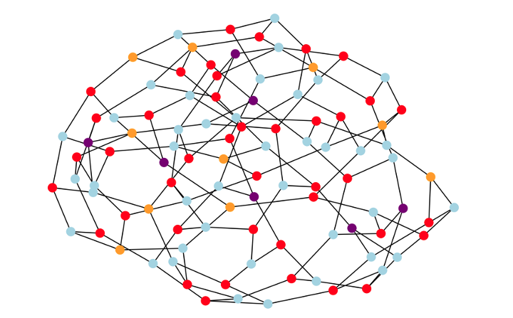
Figure 1: Example 4-coloring solution to the graph coloring problem for a random 3-regular graph with n = 100 nodes. The optimization problem is to assign the colors (in our example: red, orange, blue, and purple) in a way that adjacent nodes must be assigned different colors, while using the smallest number of colors possible (corresponding to the ground-state of the underlying antiferromagnetic Potts model).

Potts model

The GCP outlined above is closely related to the standard Potts model, a generalization of the Ising model in statistical physics. In the Potts model, every vertex is associated with a spin variable σ_i = 1, …, q that can take on q different values. The Hamiltonian for the Potts model can be expressed in compact form as:

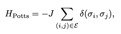
where δ(σ_i , σ_j) refers to the Kronecker delta, which equals one whenever σ_i = σ_j and zero otherwise, thus capturing the hard-core spin-spin interactions characteristic for the Potts model [2]. Accordingly, if two adjacent spins σ_i and σ_j are in the same state, the energy contribution is −J, and whenever the adjacent spins are in different states, the energy contribution is zero. To enforce a feasible coloring of the underlying graph, we consider anti-ferromagnetic interactions (i.e., with negative coupling J<0 favoring different colors for adjacent spins) and set J = −1, unless otherwise stated. The ground-state energy of the antiferromagnetic Potts model is zero if and only if the graph is q-colorable, thus providing a good cost function for encoding the GCP. Generalizations to other multi-color problems such as community detection, data clustering, and the minimum clique cover problem are straightforward, simply by considering settings with weighted interactions J -> J_ij or considering the complement of the original graph.

Relation to quantum computing

The GCP has recently attracted considerable interest in the broader quantum computing community [4, 5]. In the current era of noisy intermediate-scale quantum (NISQ) devices, typical approaches either involve hybrid quantum-classical algorithms such as the Quantum Approximate Optimization Algorithm (QAOA) or quantum annealing. In these approaches, the GCP typically has to be cast as a quadratic unconstrained binary optimization problem (QUBO [5]) or, equivalently, as an Ising Hamiltonian [6], at the expense of increased resource requirements. Specifically, the common QUBO description of the GCP with q > 2 colors for a graph with n nodes requires q × n binary variables, or (logical) qubits in the corresponding quantum-native or quantum-inspired approach. In addition, the constraint that each vertex is assigned exactly one color has to be enforced by hand via additional penalty terms [4]. For more details we refer to our previous blog post showing how to solve the closely related problem of community detection within the quantum-native QUBO formalism. As an alternative, here we propose the use of graph neural networks, guided by concepts from statistical physics.

Graph Coloring with physics-inspired graph neural networks

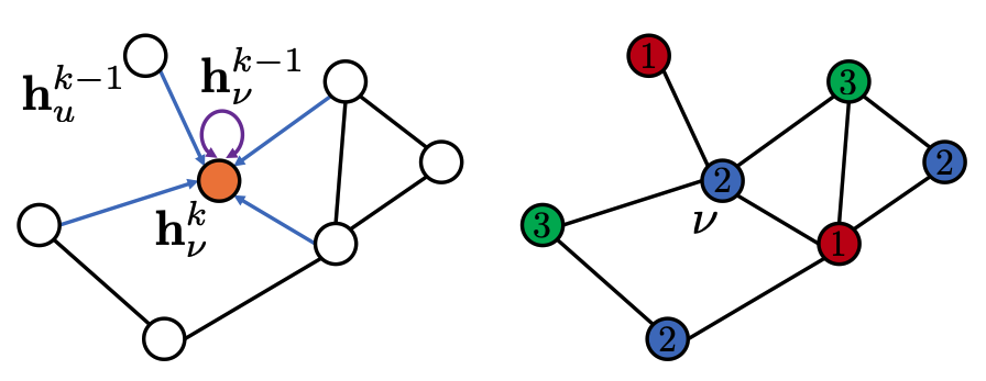
Figure 2: Schematic illustration of our approach. Following a recursive neighborhood aggregation scheme, the graph neural network is iteratively trained against a loss function based on the Potts model (enforcing different color assignments to adjacent nodes). At training completion, the values for the soft node assignments at the final graph neural network layer are projected to hard class (color) assignments σ_i = 1, …, q, as illustrated here for q = 3 colors. The shown solution for this example is optimal as the sample graph contains maximum cliques of size three.

Graph neural networks

We have previously discussed the anatomy of graph neural networks in our blog post on combinatorial optimization. There, we presented a physics-inspired, GNN-based framework to approximate quadratic unconstrained binary combinatorial optimization problems with up to millions of variables. Because of this inherent scalability and graph-based design, GNNs present a platform that can tackle the graph coloring problem at scale. In this post we generalize our framework detailed in Ref. [2] to multi-color decision variables, in particular (approximately) solving the GCP without the need for extra penalty terms as needed when using a QUBO-based approach. To this end we frame the GCP as a multi-class node classification problem and use an unsupervised training strategy based on the Potts model. The GNN is then trained to generate soft assignments to predict the likelihood of belonging in one of q classes, for each vertex in the graph. For illustration purposes, our approach is schematically depicted in Fig. 2. Note that we use the umbrella term PI-GNN (an acronym for Physics-Inspired Graph Neural Networks) to refer to our general framework, and we label our results according to the particular GNN architecture used. We include results from PI-GCN and PI-SAGE architectures, referring to popular (message-passing) implementations of GNN layers: graph convolutional networks (GCN) and Sample and AggreGatE (SAGE; as introduced in [11]). For more details, we encourage you to have a look at our original article [5].

Use case example: Scheduling

Figure 3: Example application of graph coloring for a task scheduling problem. (a), The problem is specified in terms of a schedule detailing six resource requests (vertical axis) as a function of time, spread out over the course of 24 hours (horizontal axis). (b), The problem is encoded in the form of an interval graph where every node represents one request labelled by the corresponding time interval, and edges refer to clashes within the resource requests whenever two requests overlap in time. (c), We solve the graph coloring problem on this interval graph using a graph neural network with a Potts-type loss function. Once the algorithm has converged, we obtain a graph colored with the smallest number of color clashes for the given number of colors. In this example we find a feasible coloring with χ = 3 colors as expected based on the clique of size three. (d), Finally the proposed colors are mapped back to the original resource requests. In this example we find that three resources are sufficient in order to satisfy all requests.

The graph coloring problem is known to describe many real-world applications, in particular in scheduling and allocation tasks. To illustrate both our GNN-based approach as well as the real-world applicability of the graph-coloring problem, we now discuss an end-to-end application for a canonical scheduling use case. For the sake of this illustrative example, we consider a small and simple problem instance as illustrated in Fig. 3.

We consider a scenario involving the scheduling of tasks with given start and end times, with applications in car-sharing, taxi companies, aircraft assignments, etc. Specifically, we face n resource requests (or bookings) with a start time indicating when the resource will be needed, and an end time indicating when the resource is available again; see Fig. 3(a) for an example problem with n = 6 resource requests. The problem is then to assign resources (e.g., cars) to these requests (e.g., bookings) in the most efficient way (i.e., requiring the smallest number of resources). As illustrated in Fig. 3(a), typically some requests will overlap in time leading to request clashes that cannot be satisfied by the same resource. As is commonly done in resource allocation problems and scheduling theory, this situation can conveniently be described with the help of an undirected interval graph, in which a vertex is introduced for every request, with edges connecting vertices whose requests overlap. Figure 3(b) displays an encoding of the problem with a graph made of six vertices and six edges, including a clique of size three. While inexpensive, special-purpose algorithms exist for interval graphs [1]; we can then solve the graph coloring problem on this interval graph (in the same way as any other GCP) using our general-purpose GNN-based approach. To this end, we run unsupervised multiclass classification directly on the interval graph with n = 6 nodes and use a final softmax non-linearity of dimension q = 3, as opposed to QUBO-based approaches involving q × n = 18 binary variables. For the sample problem illustrated in Fig. 3(c) we obtain a feasible coloring using just three colors (χ = 3). If no feasible solution is found, we can try to purify the solution through postprocessing routines [7] or just rerun the experiment with q=4, 5, … etc. until a feasible solution is found. Finally, as shown in Fig. 3(d), we decode this coloring to the corresponding assignment, in which three resources are used to satisfy all six requests.

Benchmark experiments

Table I: Numerical results for COLOR graph benchmark instances [8]. For a given number of colors q, we report the number of conflicts in the best coloring result, as achieved with our physics-inspired GNN solvers (dubbed PI-GCN and PI-SAGE), together with results for the Tabucol algorithm, as partially sourced from Ref. [10]. Upper bounds on the chromatic number χ as found by a greedy algorithm as well as PI-SAGE are reported as χ̄_greedy and χ̄_GNN, respectively. Best results are marked in boldface. The last column gives the normalized error (for the best PI-GNN result) specifying the relative fraction of edges with color clashes.

Table II: Numerical results for citation graph benchmark instances [9]. Columns have the same meaning as in Table I above. NA means that no solution was found within a 24h time limit [10].

For a given graph and a fixed number of colors q, we report the total number of color clashes as achieved with our physics-inspired GNN solvers (dubbed PI-GCN and PI-SAGE, respectively), and we assess the solution quality with the normalized error = H_Potts/|E| quantifying the number of color clashes normalized by the number of edges |E|. In addition, we report upper bounds on the chromatic number, denoted as χ̄_GNN, based on a simple search as well as randomized post-processing heuristic.

Our numerical results are summarized in Tab. I and II. We consistently find sub-one-percent normalized errors (i.e., < 1%) across all COLOR instances, some of which have been deemed hard, with the GraphSAGE-based architecture typically outperforming the GCN-based baseline architecture. We also find that PI-SAGE provides results comparable to traditional approaches such as Tabucol and greedy algorithms.

The scalability of our approach is illustrated in results for publicly available, real-world citation graphs, with up to n ∼ 2 × 10⁴ nodes (see Tab. II). As expected, greedy algorithms perform very well for these sparse instances, while displaying limitations for denser problems (as observed in Tab. I). At the same time, Tabucol performs well for these dense problems, while showing limitations in scalability (as reported in Tab. II). Thus, overall we see that our PI-GNN solvers may offer an alternative algorithmic approach complementing established algorithms such as Tabucol and greedy algorithms, while incorporating concepts from statistical physics and thus ultimately helping our customers understand some of the possibilities and challenges faced by quantum computing. Specifically, framing the GCP as a Potts (or the related Ising) model can help our customers build up physics literacy and ultimately quantum readiness in that it pinpoints the resource requirements for a given problem. For example, the quantum-native QUBO description (that is compatible with standard quantum annealing or QAOA) of the GCP with q > 2 colors for a graph with n nodes requires q × n binary variables, or (logical) qubits in the corresponding quantum-native approach. In addition, the constraint that each vertex is assigned exactly one color has to be enforced by hand with additional penalty terms [5, 6]. Thus, it is interesting to develop alternative approaches that tackle the problem in its native Potts mathematical form as done here with graph neural networks.

Conclusion

We have shown how graph neural networks can be used to solve graph coloring problems leveraging concepts from statistical physics as our guiding principle. In our approach we frame graph coloring as a multi-class (multi-color) node classification problem, with the Potts model providing a canonical choice for the loss function with which we train the GNN. The framework established by the Potts model provides straightforward connections to a larger class of multi-class problems, including (for example) community detection, data clustering, and the minimum clique cover problem, as relevant for the optimization of the number of measurements on quantum hardware [13].

With today’s quantum hardware still in its infancy, it is important to develop optimization methods that help establish physics literacy but can bridge the gap until quantum hardware has matured into a commercially viable technology. These may be used today to solve (large-scale) combinatorial optimization problems, while helping our customer get quantum-ready. For further technical details on this work, please check out our paper published in Physical Review Research [arXiv:2202:01606]. If your company deals with similar optimization problems and is looking for novel ways to solve them, we encourage you to reach out to the Amazon Quantum Solutions Lab to start a conversation.

References

[1] R. M. R. Lewis, A Guide to Graph Colouring – Algorithms and Applications (Springer, Heidelberg, 2016).

[2] M. J. A. Schuetz, J. K. Brubaker, and H. G. Katzgraber, Nat. Mach. Intell. 4, 367 (2022), arXiv:2107.01188.

[3] F. Y. Wu, The Potts model, Rev. Mod. Phys. 54, 235 (1982). Wikipedia article: https://en.wikipedia.org/wiki/Potts_model.

[4] Y.-H. Oh, H. Mohammadbagherpoor, P. Dreher, A. Singh, X. Yu, and A. J. Rindos, Solving MultiColoring Combinatorial Optimization Problems Using Hybrid Quantum Algorithms, arXiv:1911.00595.

[5] F. Glover, G. Kochenberger, and Y. Du, Quantum Bridge Analytics I: A Tutorial on Formulating and Using QUBO Models, 4OR 17, 335 (2019).

[6] A. Lucas, Ising formulations of many NP problems, Front. Physics 2, 5 (2014).

[7] M. J. A. Schuetz, J. K. Brubaker, Z. Zhu, and H. G. Katzgraber, Phys. Rev. Research 4, 043131 (2022).

[8] M. Trick, COLOR Dataset, URL (2002), https://mat.tepper.cmu.edu/COLOR02/.

[9] A. K. McCallum, K. Nigam, J. Rennie, and K. Seymore, Automating the construction of internet portals with machine learning, Information Retrieval 3, 127 (2000). P. Sen, G. Namata, M. Bilgic, L. Getoor, B. Galligher, and T. Eliassi-Rad, Collective classification in network data, AI magazine 29, 93 (2008). G. Namata, B. London, L. Getoor, and B. Huang, in 10th International Workshop on Mining and Learning with Graphs (2012), vol. 8, p. 249.

[10] W. Li, R. Li, Y. Ma, S. On Chan, and B. Yu, Rethinking Graph Neural Networks for Graph Coloring (2021), (ICLR 2021 Conference Withdrawn Submission).

[11] W. Hamilton, Z. Ying, and J. Leskovec, in Advances in neural information processing systems (2017), p. 1024.

[12] A. Hertz and D. de Werra, Using tabu search techniques for graph coloring, Computing 39, 345 (1987).

[13] J. Izaac, Measurement optimization, https://pennylane.ai/qml/demos/tutorial_measurement_optimize.html.