Combinatorial Optimization with Physics-Inspired Graph Neural Networks

Combinatorial optimization problems, such as the traveling salesman problem where we are looking for an optimal path with a discrete number of variables, are pervasive across science and industry. Practical (and yet notoriously challenging) applications can be found in virtually every industry, such as transportation and logistics, telecommunications, and finance. For example, optimization algorithms help us schedule planes and their crews, organize real-time markets to deliver electricity to millions of people, orchestrate the production of cars, and organize the transportation of these cars from the assembly lines to the car dealers.

Quantum computers hold the promise to solve seemingly intractable problems across disciplines, with simulation and optimization likely being the first medium-term workloads. While there have been substantial advances in quantum hardware over the last few years, currently the field is still in its infancy. Thus, it is imperative to develop optimization methods that can bridge the gap until quantum hardware has matured into a commercially viable technology, thereby allowing us to deliver real value to business today. Leveraging these methods also prepares our customers to become familiar with optimization models that will eventually be able to be run on quantum hardware.

In this blog we show how physics-inspired graph neural networks can be used to address these needs, solving large-scale combinatorial optimization problems with quantum-native models. Our approach is broadly applicable to canonical NP-hard problems in the form of Quadratic Unconstrained Binary Optimization (QUBO) problems, or equivalently Ising spin glasses, and provides a unifying framework that incorporates insights from statistical physics. We discuss how to frame problems in QUBO form, and how to solve these problems with both quantum annealers (as available on Amazon Braket) as well as physics-inspired graph neural networks. We show that the graph neural network optimizer we developed performs on par with or outperforms existing classical solvers, with the ability to scale beyond the state of the art to problems with millions of variables, while helping our customers get quantum-ready.

The QUBO formalism and its relation to quantum computing

QUBO model. The field of combinatorial optimization is concerned with settings where a large number of yes/no decisions must be made and each set of decisions yields a corresponding objective function value, like a cost or profit value, that is to be optimized. Canonical combinatorial optimization problems include, among others, the maximum cut problem (MaxCut), the maximum independent set problem (MIS), the minimum vertex cover problem, the maximum clique problem, and the set cover problem. In all cases, exact solutions are not feasible for sufficiently large systems due to the exponential growth of the solution space as the number of variables n increases. To solve these problems bespoke (approximate) algorithms can typically be identified, at the cost of limited scope and generalizability. Conversely, in recent years the QUBO model has resulted in a powerful approach that unifies a rich variety of these NP-hard combinatorial optimization problems. The cost function for a QUBO problem can be expressed in compact form with the following Hamiltonian:

H_QUBO​ = x^⊺Qx = ∑_i,j​x_i​Q_ij​x_j​

Where x=(x₁​,x₂​,…) is a vector of binary decision variables and the QUBO matrix Q is a square matrix that encodes the actual problem to solve. Without loss of generality, the Q-matrix can be assumed to be symmetric or in upper triangular form. We have omitted any irrelevant constant terms, as well as any linear terms, as these can always be absorbed into the Q-matrix because x_i²​=x_i​ for binary variables x_i​∈{0,1}. Problem constraints, as relevant for many real-world optimization problems, can be accounted for with the help of penalty terms entering the objective function, rather than being explicitly imposed.

Ising model. The significance of QUBO problems is further illustrated by its close relation to the famous Ising model, with Hamiltonian H_Ising​=∑_i,j​J_i,j​z_i​z_j​+∑_i​h_i​z_i​, which is known to provide mathematical formulations for many NP-complete and NP-hard problems, including all of Karp’s 21 NP-complete problems. As opposed to QUBO problems, Ising problems are described in terms of binary spin variables z_i​∈{−1,1}, that can be mapped straightforwardly to their equivalent QUBO form, and vice versa, using z_i​=2x_i​−1. Thus, solutions to the Ising model can be readily mapped to solutions of the corresponding QUBO problem, and vice versa. One particular strategy to try when solving Ising models (or equivalent QUBO models) on quantum hardware is quantum annealing.

Quantum annealing. The QUBO model (or equivalent Ising model) is quantum-native, meaning it can be directly mapped to and processed by a quantum computer. It is at the heart of quantum annealing devices, such as those available through Amazon Braket from D-Wave Systems. These devices are special purpose machines built for solving QUBO models by a process called quantum annealing , which to some extent can be seen as the quantum counterpart to classical simulated annealing–a physics-inspired approach. Here, the classical logical variables z_i​ are mapped to their quantum-mechanical counterparts, called qubits. First initialized in the ground state of a simple single-qubit driving Hamiltonian, the machine then follows through the annealing schedule, trying to adiabatically convert this easily prepared ground state to the ground state of the original QUBO model, and then upon measurement of the qubits, reading out the solution as a classical bitstring. Typically, this process is repeated many times to increase the chances for finding a high-quality solution.

Quantum annealing on Amazon Braket. To learn more about D-Wave and quantum annealing, log onto AWS and follow one of our Amazon Braket notebooks that help you get started with quantum annealing. For more detailed examples, there are two blog posts showing how to solve community detection (Part 1 & Part 2) and price optimization problems using quantum annealing on Amazon Braket.

Graph neural networks overview

Graph Neural Networks. In the deep learning community, graph neural networks (GNNs) have recently emerged as a novel class of neural network architectures designed to consume graph structure data, with the ability to learn effective feature representations of nodes, edges, or even entire graphs. Paradigmatic problems studied with GNNs can be categorized as node classification, link prediction, graph classification, or community detection, among others. Examples include the classification of users in social networks, the prediction of future interactions in recommender systems, and the prediction of certain properties of molecular graphs. The unifying theme underlying GNNs is the implementation of some form of a message passing scheme whereby GNNs iteratively update the node (or edge) embeddings by aggregating information from their local neighbors.

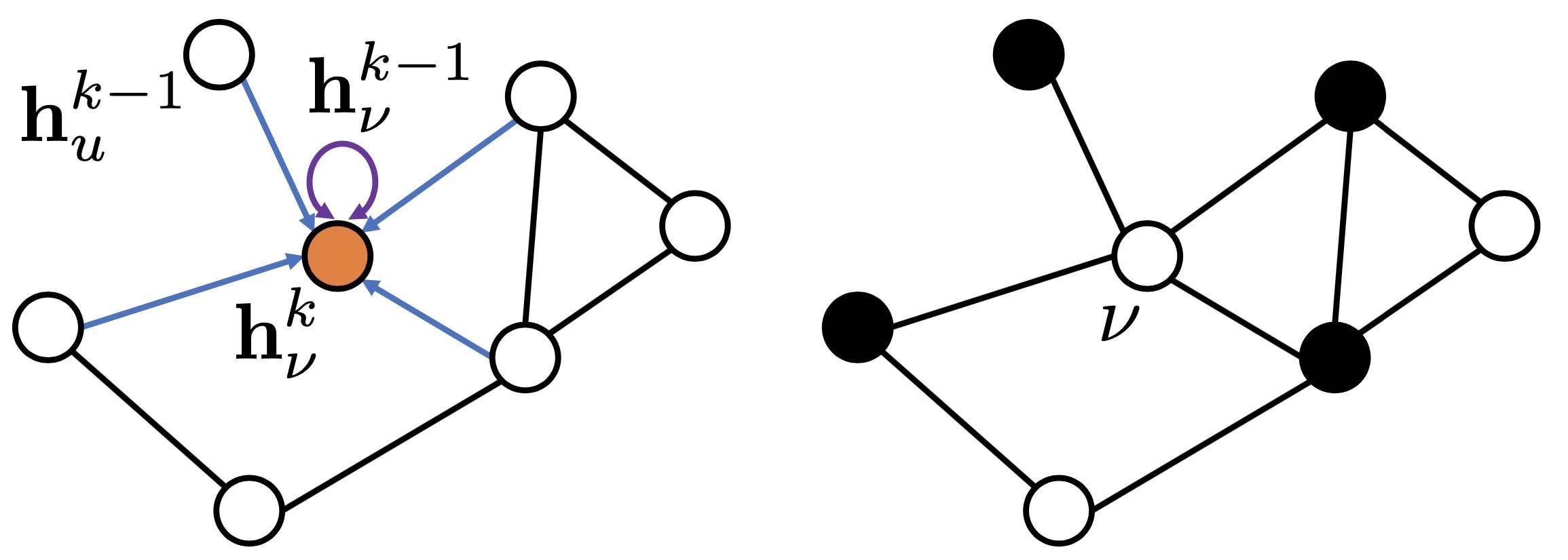
Figure 1: Schematic illustration of graph neural networks, where nodes are represented internally by embedding vectors h_v^k​ for ν=1,…,n. Following a recursive neighborhood aggregation scheme, the GNN then iteratively updates each node’s representation, as described by some learnable, parametric function.

Anatomy of graph neural networks. On a high level, GNNs are a family of neural networks capable of learning how to aggregate information in graphs for the purpose of representation learning. Typically, a GNN layer is comprised of three functions:

1. A message passing function that permits information exchange between nodes over edges.
2. An aggregation function that combines the collection of received messages into a single, fixed-length representation.
3. A (typically nonlinear) update activation function that produces node-level representations given the previous layer representation and the aggregated information.

While a single-layer GNN encapsulates a node’s features based on its immediate or one-hop neighborhood, by stacking multiple layers, the model can propagate each node’s features through intermediate nodes, analogous to broadening the receptive field in downstream layers of convolutional neural networks. Formally, at layer k=0, each node ν∈V is represented by some initial representation, h_ν⁰​∈R^d₀​, usually derived from the node’s label or given input features of dimensionality, d₀​. Following a recursive neighborhood aggregation scheme, the GNN then iteratively updates each node’s representation, in general described by some parametric function, f_θ^k​, resulting in:

h_ν^k ​= f_θ^k​(h_ν^k−1​, {h_u^k−1​∣u∈N_ν​})

For the layers k=1,…,K, with N_ν​={u∈V∣(u,ν)∈E} referring to the local neighborhood of node ν, i.e., the set of nodes that share edges with node ν. The total number of layers, K, is usually determined empirically as a hyperparameter, as are the intermediate representation dimensionality, d_k​; both can be optimized in an outer loop.

Physics-inspired graph neural networks for combinatorial optimization

Because of their inherent scalability and graph-based design, GNNs provide a platform poised to solve optimization problems at scale. Specifically, our key idea is to frame combinatorial optimization problems as unsupervised node classification tasks whereby the GNN learns color (in other words, spin) assignments for every node. To this end, the GNN is iteratively trained against a custom loss function that encodes the specific optimization problem of interest.

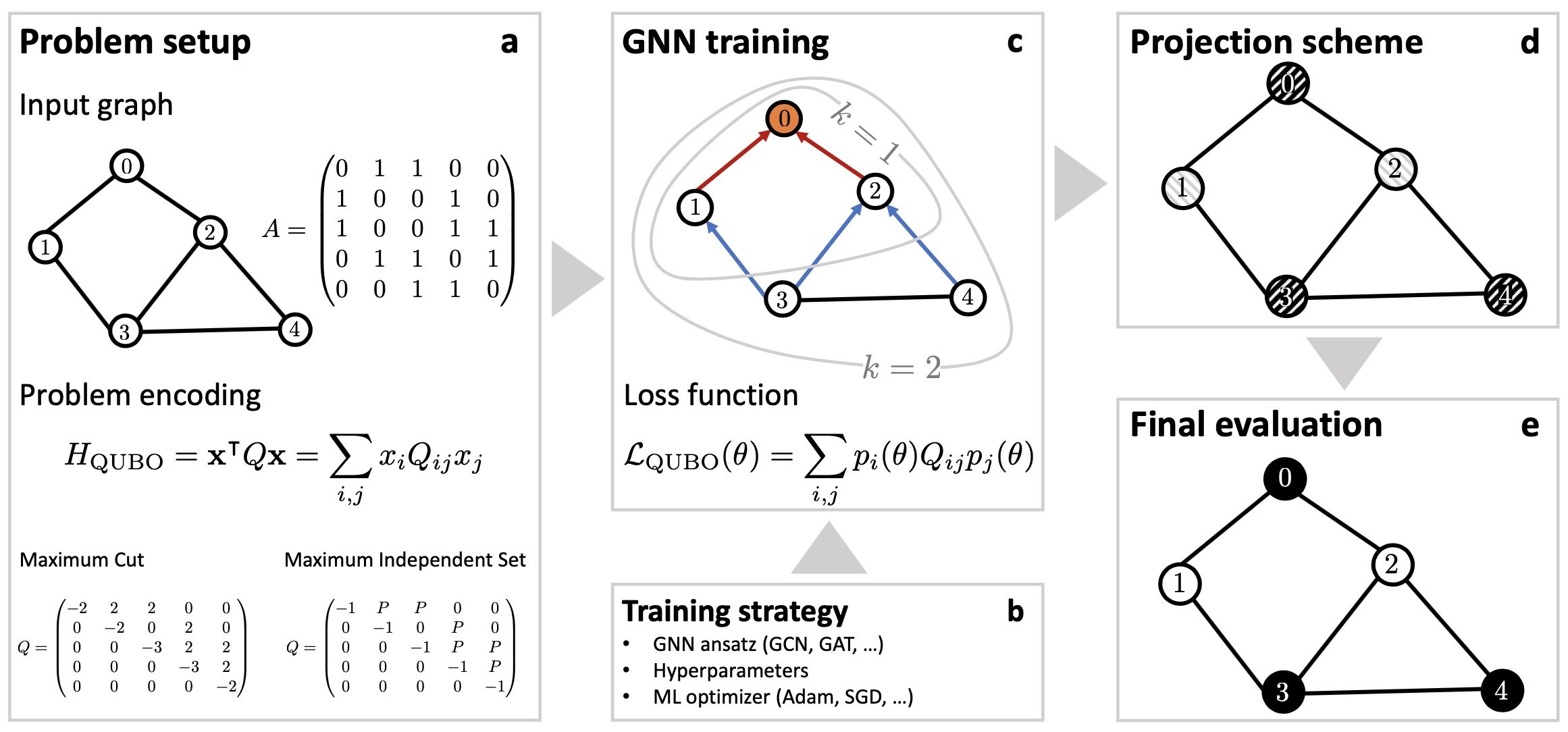
Figure 2:  Flow chart illustrating the end-to-end workflow for the physics-inspired GNN optimizer. Following a recursive neighborhood aggregation scheme, the graph neural network is iteratively trained against a custom loss function that encodes the specific optimization problem (e.g., maximum cut, or maximum independent set). At training completion, we project the final values for the soft node assignments at the final graph neural network layer back to binary variables x_i​∈{0,1} (as indicated by the binary black/white node coloring), providing the solution bit string x=(x₁, x₂,…).

Physics-inspired graph neural networks. The end-to-end workflow for the physics-inspired GNN optimizer is schematically depicted in Figure 2, and works as follows:

(a) The problem is specified by a graph G with associated adjacency matrix A, and a cost function as described by the QUBO Hamiltonian H_QUBO​. Within the QUBO framework the cost function is fully captured by the QUBO matrix Q, as illustrated for both MaxCut and MIS for a sample undirected graph with five vertices and six edges.

(b) The problem setup is complemented by a training strategy that specifies the GNN Ansatz, a choice of hyperparameters and a specific ML optimizer.

(c) The GNN is iteratively trained against a custom loss function L_QUBO​(θ) that encodes a relaxed version of the underlying optimization problem as specified by the cost function H_QUBO​. Typically, a GNN layer operates by aggregating information within the local one-hop neighborhood (as illustrated by the k=1 circle for the top node with label 0). By stacking layers one can extend the receptive field of each node, thereby allowing distant propagation of information (as illustrated by the k=2 circle for the top node with label 0). Specifically, the GNN follows a standard recursive neighborhood aggregation scheme, where each node i=1,2,…,n collects information (encoded as feature vectors) of its neighbors to compute its new feature vector h_i^k​ at layer k=0,1,…,K.

(d) – (e) The GNN generates soft node assignments, which can be viewed as class probabilities. Specifically, for binary classification tasks we typically use convolutional aggregation steps, followed by the application of a nonlinear softmax activation function to shrink down the final embeddings h_i^K to one-dimensional soft (probabilistic) node assignments p_i​=h_i^K​∈[0,1]. Using some projection scheme, for example, x_i​=int(p_i​), we then project the soft node assignments back to hard binary variables x_i​ = 0,1 (as indicated by the binary black/white node coloring), providing the final solution bit string x.

Next, we review how our physics-inspired GNN solver can be used to solve real world examples via their construction as maximum independent set problems.

Use case examples: From portfolio management and machine scheduling to the maximum independent set problem

Risk diversification. To introduce how the field of combinatorial optimization maps to real-world problems, let us start out with an illustrative example, and consider the following portfolio management problem. Specifically, here we outline a risk diversification strategy, but similar considerations apply for the implementation of hedging strategies. We consider a (potentially very large) universe of n assets, for which we are given the covariance matrix Σ∈R^n×n capturing volatility through the correlations among assets. To minimize the volatility of our portfolio, our goal is to select a subset of uncorrelated assets with the largest possible diversified portfolio. To this end, we consider a graph G with n nodes, with every node representing one asset. Correlations can be described in graph form, either by directly taking the cross-correlation matrix as a weighted adjacency matrix, or by creating a binary adjacency matrix A through thresholding. Here, we set A_i,j​=1 if and only if the absolute value of the correlation between assets i and j is greater than some user-specific threshold parameter λ, and A_i,j​=0 otherwise [1]. Accordingly, in our model, pairs of assets are classified as correlated or uncorrelated based on whether or not the corresponding correlation coefficient exceeds a minimum level. Overall, the risk diversification strategy outlined earlier can then be cast as an optimization problem, as described by the Hamiltonian:

H_MIS = -∑_i∈V x_i + P ∑_(i,j)∈E x_ix_j

By minimizing H_MIS​ we select the largest possible number of uncorrelated assets, as captured by the independent set constraint with a positive pre-factor P>0. Such a diversification model could be part of a larger, two-stage portfolio management pipeline where first a subset of assets is selected from a larger universe of assets, and then capital is allocated within a smaller, sparsified basket of assets using some off-the-shelf solvers.

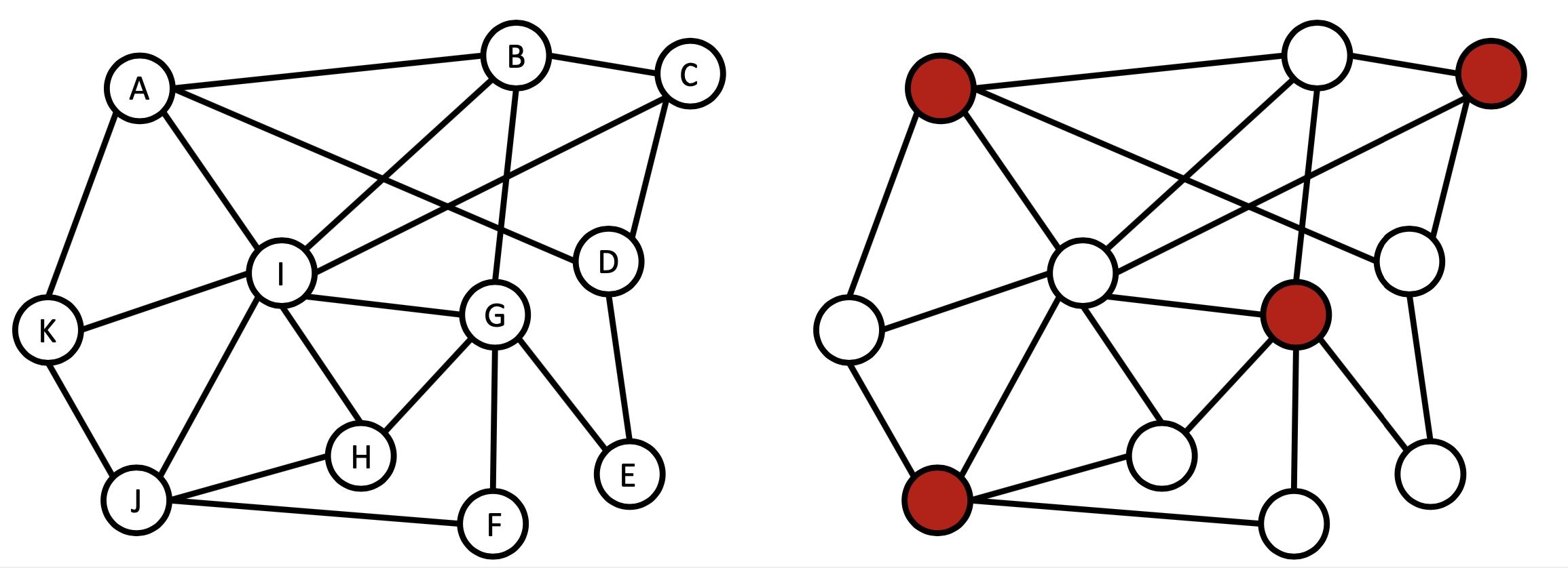
Figure 3: Example application of the MIS problem for a risk diversification problem, with n=11 assets, labelled as A, B, …, K. (a), The problem described by a graph with n=11 nodes and edges describing correlations between assets, i.e., non-adjacent nodes refer to uncorrelated assets, and adjacent nodes refer to correlated assets. (b), Finding the largest basket of uncorrelated assets amounts to finding the maximum independent set (MIS) in this graph. The solution highlighted in red suggests investing in the four uncorrelated assets A, C, G, and J. Similar considerations apply to hedging strategies.

Interval scheduling. Next, let us consider a scenario involving the scheduling of tasks with given start and end times, as relevant, for example, in the context of the scheduling of jobs on machines (resources). Specifically, we face n resource requests, each represented by an interval specifying the time in which it needs to be processed by some machine. Typically, some requests will overlap in time leading to request clashes that cannot be satisfied by the same machine. Conversely, a subset of intervals is deemed compatible if no two intervals overlap on the machine. As commonly done in resource allocation problems, this situation can conveniently be described with the help of an undirected interval graph G in which we introduce a vertex for each request and edges between vertices whose requests overlap, as shown in the figure earlier. With the goal to maximize the throughput (i.e., to execute as many tasks as possible on a single machine), the interval scheduling maximization problem is then to find the largest compatible set, that is, a set of non-overlapping intervals of maximum size. This use case turns out to be equivalent to finding the maximum independent set (MIS) in the corresponding interval graph G with n nodes; mathematically it is described by the very same Hamiltonian as discussed earlier in the context of risk diversification.

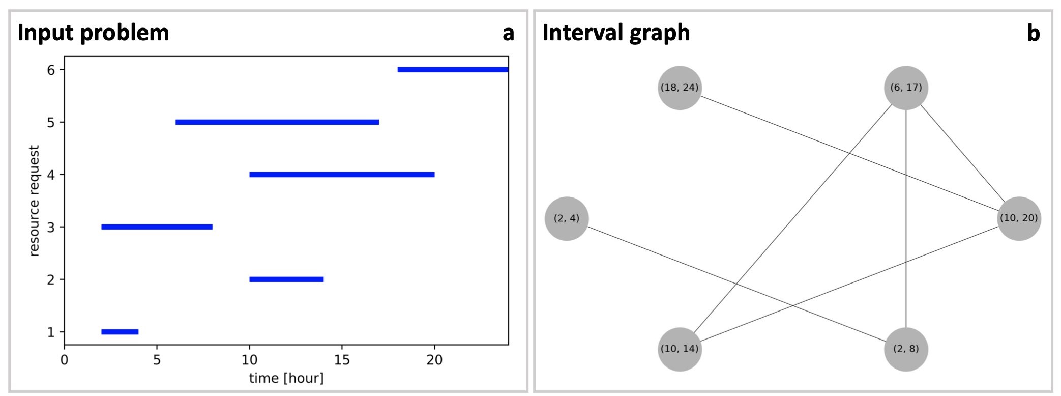
Figure 4: Example application of the MIS problem for a task scheduling problem. (a) The problem is specified in terms of a schedule detailing six resource requests (vertical axis) as a function of time, spread out over the course of 24 hours (horizontal axis). (b) The problem is encoded in the form of an interval graph where every node represents one request labelled by the corresponding time interval, and edges refer to clashes within the resource requests whenever two requests overlap in time. The interval scheduling maximization problem, with the goal to execute as many requests as possible on a single machine, amounts to finding the maximum independent set (MIS) in this interval graph.

Maximum independent set problem. The two use cases outlined earlier map onto the very same combinatorial optimization problem, known as the maximum independent set problem. The MIS problem is a prominent (NP-hard) combinatorial optimization problem, making the existence of an efficient algorithm for finding the maximum independent set on generic graphs unlikely. In the quantum community, the MIS problem has recently attracted significant interest [2] as a potential target use case for novel experimental platforms based on neutral atom arrays [3]. For more details on analog Hamiltonian Rydberg simulators we refer to this blog post.

More formally, the MIS problem reads as follows: given an undirected graph G=(V,E), an independent set is a subset of vertices that are not connected with each other. The MIS problem is then the task to find the largest independent set, with its (maximum) cardinality typically denoted as the independence number α. To formulate the MIS problem mathematically, for a given graph G=(V,E), one first associates a binary variable x_i​∈{0,1} with every vertex i∈V, with x_i​=1 if vertex i belongs to the independent set, and x_i​=0 otherwise. The MIS can then be formulated in terms of a Hamiltonian H_MIS​ that counts the number of marked (colored) vertices and adds a penalty to nonindependent configurations (when two vertices in this set are connected by an edge), as given above. A negative pre-factor is applied to the first term, because we solve for the largest independent set within a minimization problem, and the penalty parameter is defined as P>0, enforcing the constraints. The numerical value for P is typically set as P=2, but can be further optimized in an outer loop. Energetically, the Hamiltonian H_MIS​ favors each variable to be in the state x_i​=1 unless the pair are connected by an edge.

Benchmark experiments for the maximum independent set problem

Benchmarking for MIS. To numerically validate our approach, we study the MIS problem on random unweighted d-regular graphs. For small graphs with up to a few hundred nodes, we compare the GNN-based results to results obtained with the Boppana-Halldorsson algorithm built into the Python NetworkX library. For very large graphs with up to a million nodes (where benchmarks are not available) we resort to analytical upper bounds for random d-regular graphs as presented in Ref. [4]. Here, the best known bounds on the ratio α_d​/n are reported as α₃​/n=0.45537 and α₅​/n=0.38443 for d=3 and d=5, respectively, as derived using refined versions of Markov’s inequality. Our results for the achieved independence number as a function of the number of vertices n are shown in Figure 5. For graphs with up to a few hundred nodes, we find that a simple two-layer GCN architecture can perform on par with (or better than) the traditional solver, with the physics-inspired GNN solver showing a favorable runtime scaling. For large graphs with n≈10⁴−10⁶ nodes we find that our approach consistently achieves high-quality solutions with estimated numerical approximation ratios of ∼0.92 and ∼0.88, respectively. Finally, we observe a moderate, super-linear scaling of the total runtime as ∼n^1.7 for large d-regular graphs with n≳10⁵, as opposed to the Boppana-Halldorsson solver with a runtime scaling of ∼n^2.9 in the range n≲500. Note that the GNN model training alone displays sub-linear runtime scaling as ∼n^0,8, while the aggregate runtime (including post-processing to enforce the independence condition) scales as ∼n^1.7 in the regime n∼10⁵−10⁶.

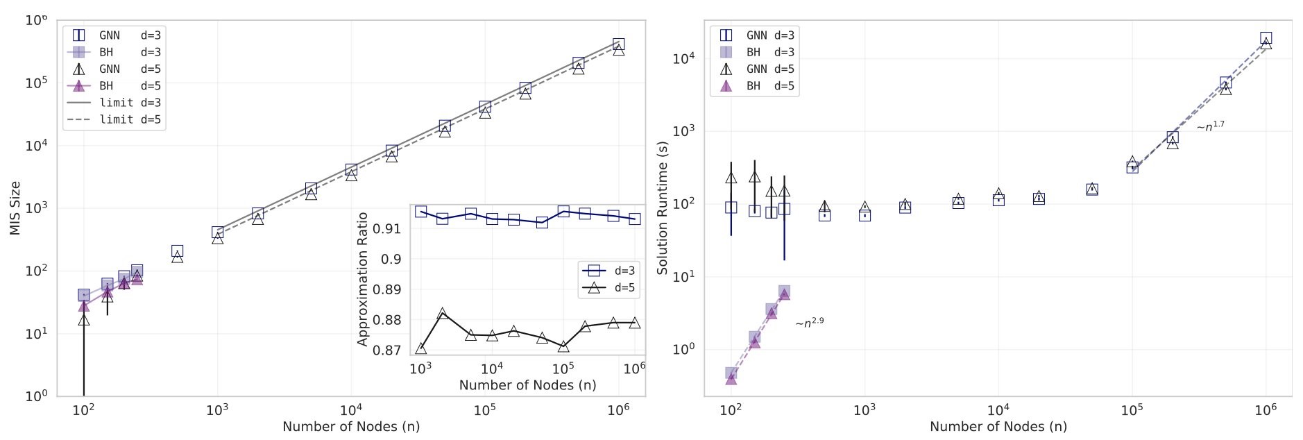
Figure 5: Numerical results for the MIS problem for up to 10⁶ nodes (variables). (Left) Average independence number for d-regular graphs with d=3 and d=5 as a function of the number of vertices n, bootstrap-averaged over 20 random graph instances, for both the GNN-based method and the traditional Boppana-Halldorsson (BH) algorithm. Solid lines for n≥10³ refer to theoretical upper bounds as described in the main text. Inset: The estimated relative approximation ratio comparing the achieved independence number α against known theoretical upper bounds shows that our approach consistently achieves high-quality solutions. (Right) Algorithm runtime in seconds for both the GNN solver and the BH algorithm. Error bars refer to twice the bootstrapped standard deviations, sampled across 20 random graph instances for every data point.

Conclusion

In this post we have shown how to frame real-world optimization problems taken from portfolio management and machine scheduling as maximum independent set (MIS) problems. We saw that this MIS problem falls into the larger class of quantum-native QUBO, or equivalently Ising, problems. This is the appropriate modeling framework both for quantum annealers or the hybrid quantum approximate optimization algorithm (QAOA), running on gate-based quantum computer, as available today on Amazon Braket. With today’s quantum hardware still in its infancy, it is important to develop optimization methods that can bridge the gap until quantum hardware has matured into a commercially viable technology. To this end, we have outlined the anatomy of physics-inspired graph neural networks. These can be used today to solve (large-scale) combinatorial optimization problems with quantum-native models, thus helping our customers get quantum-ready. The scalability of our approach opens up the possibility of studying unprecedented problem sizes with hundreds of millions of nodes when leveraging distributed training in a mini-batch fashion on a cluster of machines as demonstrated recently in Ref. [5]. For those interested in taking a deeper dive into solving combinatorial optimization problems with graph neural networks, please refer to our work published in Nature Machine Intelligence. If you deal with large and complex optimization problems and are interested in exploring new solutions, such as with our GNN-based approach, we encourage you to reach out to the Amazon Quantum Solutions Lab to start a conversation.

References

[1] A. Kalra, F. Qureshi, and M. Tisi, Portfolio Asset Identification Using Graph Algorithms on a Quantum Annealer, SSRN (2018), URL https://ssrn.com/abstract=3333537.

[2] H. Yu, F. Wilczek, and B. Wu, Quantum Algorithm for Approximating Maximum Independent Sets, arXiv:2005.13089.

[3] H. Pichler, S.-T. Wang, L. Zhou, S. Choi, and M. D. Lukin, Quantum Optimization for Maximum Independent Set Using Rydberg Atom Arrays, arXiv:1808.10816.

[4] W. Duckworth and M. Zito, Large independent sets in random regular graphs, Theoretical Computer Science 410, 5236 (2009).

[5] D. Zheng, C. Ma, M. Wang, J. Zhou, Q. Su, X. Song, Q. Gan, Z. Zhang, and G. Karypis, DistDGL: Distributed Graph Neural Network Training for Billion-Scale Graphs, arXiv:2010.05337.