Using quantum annealing on Amazon Braket for price optimization

Combinatorial Optimization is one of the most popular fields in applied optimization, and it has various practical applications in almost every industry, including both private and public sectors. Examples include supply chain optimization, workforce and production planning, manufacturing layout design, facility planning, vehicle scheduling and routing, financial engineering, capital budgeting, retail seasonal planning, telecommunication network design, and many more.

At a high level, combinatorial optimization [1] aims at finding an optimal solution from a finite set of solutions, where the set of feasible solutions is discrete. However, finding an optimal solution from a finite set of possible solutions or even sufficiently good solutions can be extremely difficult. First, traditional approaches are usually tailored to specific use-cases based on the particular mathematical structure of each use-case. In addition, most combinatorial optimization problems are NP-hard, and the pool of candidate solutions is usually growing exponential in any real-world scenario, with extensive requirements for computational resources and run-times.

In this blog, we use a general-purpose mathematical formulation, Quadratic Unconstrained Binary Optimization (QUBO), which has been proposed as an effective optimization formulation that can generalize across a large variety of combinatorial optimization use cases in industry [2, 3].

QUBO basics

The formal definition of a QUBO is strikingly simple:

Minimize:where x is a vector of binary variables representing the decision variables of the combinatorial optimization. Q is a square matrix of constants inherently encoding the context and constraints of the optimization problem (Q is commonly assumed to be symmetric or upper triangular without loss of generality). The goal is to find the optimal values of the binary decision variables x that minimize the objective H.

In the following paragraphs, we take price optimization as an example and showcase how it can be casted to QUBO formulation and solved with a quantum annealer on Amazon Braket – the quantum computing service of AWS. Finally, we discuss and explore the trade-off between maximizing revenue and minimizing risk in the price optimization use case.

The notebook implementation of this use case can be found here.

Overall objective function

The overall objective function incorporates the following effects:

maximizing the expected revenue R
minimizing the prediction uncertainty
equality constraints ensuring price to be selected from a predefined set of discrete price values

Therefore, the Hamiltonian to minimize can be represented as

where R is the expected total revenue of the next n days, T simply represents tomorrow, var(d^᷍_t) is the estimated variance of the predicted demand d_t at day t. β is a hyperparameter to control the trade-off between maximizing revenue and minimizing uncertainty. H_p is a penalty term transformed from the equality constraints.

The Expected Revenue

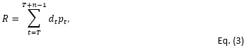
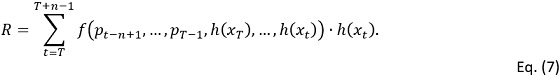
The goal of this use case is to find the optimal prices (of a set of assets, commodities, products, etc.) for each day in a specified period of time (n days) in the future, such that we maximize the total revenue over that period. Assuming tomorrow is day T, then the total revenue can be represented as:

here,

R is the total revenue we want to maximize over the next n days.
d_t is the demand of the target product at day t, t ∈ [Τ,Τ + 1, … , Τ + n – 1], which can be represented as a function of prices p.
p_t is the price value of that product at day t.

For this use case, we assume that the price at a certain day can only be a value selected from a fixed set of discrete price options [c₀, c₁, …, c_m-1].

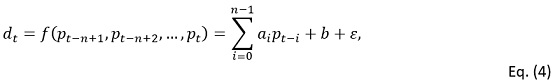
The demand d_t at day t is assumed as a linear function of the last n days’ prices. Here for convenience, we assume this number n equals to the number n of future days we want to maximize the revenue for as in Eq. (3), i.e.,

where

a_i, i ∈ [0,1, … , n – 1] are the coefficients between prices at day [t, t – 1, … , t – n + 1], and the demand d_t at day t, respectively,
b is a constant.
ε is a zero-mean Gaussian random variable with variance σ²representing the demand shocks.

In a real world example, the coefficients can be estimated from historical pricing data:

P = [p₁, p₂, … , p_T-1]
Y = [d₁, d₂, … , d_T-1].

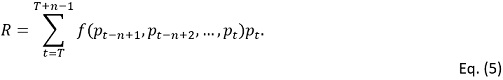
Therefore, the projected revenue R in Eq. (3) can be estimated as a function of price variables

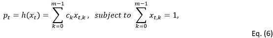
Our next step is to transform this model into a QUBO. To do this, we must identify the binary decision variables. In this use case, the possible prices are defined to be a set of discrete price values (e.g. $5.99, $9.99, $14.99, etc). Therefore, the price p_t at a certain day t can only be one value selected from this set. We can encode the next n days’ price variable p_t (for t ∈ [T, T + 1, … , T + n-1]) by a set of binary variables:

where

c_k,k ∈ [0, 1, … , m – 1] are the m available discrete price values.
x_t,k is the binary decision variable with 1 indicating that p_t equals c_k and 0, otherwise.
x_t= [x_t,0, … , x_t,m-1] represents the vector of binary decision variables for day t.

By substituting the next n days’ prices with binary variables x_t, the revenue R in Eq. (5) can be rewritten as:

With the help of the open-source library pyqubo [7], we can easily define these binary variables and represent price, demand, and revenue accordingly.

from pyqubo import Binary
days = len(a) # next number of days to optimize
n_level = len(price_levels)  # number of price options

x = []
p = []
# get prices
for t in range(days):
    p_t = 0
    for k in range(n_level):
        x_tk = Binary(f"X_{t*n_level+k}")
        x.append(x_tk)
        p_t += x_tk*price_levels[k]
    p.append(p_t)

# get demand…
def get_demand(coeff, b, prices):
    assert len(coeff) == len(prices)
    d = b
    for i in range(len(coeff)):
        d += coeff[i]*prices[i]

    return d

# get revenue…
def get_demands_rev(a,b,hist_p, p):
# hist_p: last n days prices [T-n, …, T-1] 
# p: next n days prices [T, …, T+n-1]
    all_p = hist_p + p
    n = len(a)
    d = []
    rev = 0
    for i in range(n):
	 # Get demand at T+i
        d_i = get_demand(
            coeff=a,
            b=b,
            prices=all_p[i+1:i+1+n]
        )
        d.append(d_i)
        # get revenue at T+i
        rev += d_i * p[i]
    return d, rev

Prediction Uncertainty

As the future demand values can only be estimated (thereby introducing uncertainty into our model), it is desirable to control the uncertainties/risk while maximizing the expected revenue [5,6]. As shown in the objective function, we use the estimated variance of the demand prediction to represent the uncertainties,

where

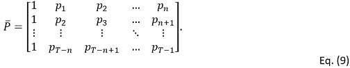
p̄_t=[1, p_t-n+1, p_t-n+2, …, p_t] is the vector of price variables.
P̄ is the historical price observations used to fit the demand model. Specifically,

The residual variance, σ², is given by

where â = [b, α₀, α₁, … , α_n-1] is the vector of price coefficients with constant b. As we can see, this demand prediction uncertainty var(d̂_t) is a quadratic form of price variables p̄_{t ,} and hence, it is also a quadratic form of binary variables [x_T, …, x_t]. Thus,var(d̂_t) falls within QUBO framework.

Incorporate equality constraints

As shown in Eq. (6), when we transform the price p_t to binary variables x_t, equality constraints are imposed to ensure that the price can only take one choice from a set of discrete price options on a given day.

The equality constraints read: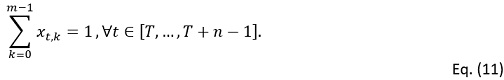As a QUBO is naturally an unconstrained optimization formulation, we incorporate these equality constraints into the objective function with the help of so-called penalty terms. The penalty terms are zero if the corresponding constraint is satisfied and larger than zero otherwise. We introduce a large penalty to the objective function if the constraints are violated. Thus,

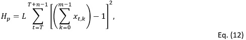where L is a large constant. The penalty term evaluates to 0 only if all the equality constraints are satisfied.

Therefore, the objective function H in Eq. (2) can be represented by a set of binary variables [x_T, … , x_T+n-1] using the pyqubo library as shown earlier. It can then be transformed to QUBO format H = x^TQx with a single line of code. We also include a minus sign in the objective function of the QUBO to align with energy minimization in physics.

# objective is the objective function represented by pyqubo Binary

model = (-objective).compile().to_bqm()
pp.pprint(model)

BinaryQuadraticModel(   {   'X_000': -10000000001058.88,
                            'X_001': -10000000001606.432,
                            'X_002': -10000000001934.893,
                            'X_003': -10000000002234.094,
                            …,
				},
                        {   ('X_000', 'X_003'): 20000000000438.887,
                            ('X_000', 'X_004'): 20000000000475.457,
                            ('X_000', 'X_007'): 80.80706691928134,
                            ('X_000', 'X_010'): 193.9369606062752,
                            ('X_000', 'X_013'): 307.06685429326905,
                            ('X_000', 'X_015'): 119.19234226406782,
                            ('X_000', 'X_019'): 238.38468452813564,
                            …,
				},
                        70000000000715.1,
                        'BINARY')

Minimizing QUBOs on Amazon Braket

Amazon Braket for QUBO problems

We use Amazon Braket to solve our QUBO Model. Amazon Braket provides access to quantum annealers from D-Wave Systems Inc. A quantum annealer is a specialized quantum device that solves combinatorial optimization problems by taking advantage of quantum fluctuations and quantum tunneling to escape local minima in complex energy landscapes [4]. Through an Amazon Braket API call, the formatted QUBO problem can be embedded into the hardwired topology of the D-Wave device and submitted to the device for execution. In turn, the quantum annealer performs an annealing process and obtains a result. However, because of the sparsity of the underlying chip, one typically faces overhead in embedding the original QUBO problem into the D-Wave hardware. Typically, one logical binary variable maps onto several physical qubits in the device, since the original QUBO problem is often more densely connected than the underlying device topology. For more details, we refer to the Amazon Braket tutorial notebook available here.

How to solve QUBOs on Amazon Braket

Train demand forecast model

As discussed in the optimization objective function Eq. (2), we must train a demand forecast model in order to formulate the objective function of our QUBO problem. Using Amazon SageMaker, we can easily use the sklearn library to train a linear demand forecast model based on the dataset of historical observations on prices P and demands Y. Then, the estimators of the price coefficients â_j, j ∈ [0, 1, … , n – 1] and constant b̂ can be obtained.

from sklearn.linear_model import LinearRegression
reg = LinearRegression().fit(data_x, data_y)
a = reg.coef_
b = reg.intercept_

Construct and solve QUBO on Amazon Braket

To use Amazon Braket, we first create a notebook instance through the Amazon Braket console. From the instance, the QUBO task will be sent through an API call to the D-Wave QPU, where the quantum annealer will solve the QUBO and send the result back to the Amazon Braket notebook. All results will also be stored in Amazon S3.

With the trained linear demand forecast model, we can derive and represent our objective function and transform it to the QUBO format using the pyqubo library. Then, we can use the Amazon Braket Python SDK to embed and submit the QUBO task to be solved by a D-Wave QPU. Similar to classical simulated annealing, we take several independent shots in order to increase our chances of success in finding a high-quality solution to the QUBO problem. The response contains a number of rows. Each row represents the optimization result of a single shot, including the binary decision variables [x_T, … , x_T+n-1], and the corresponding energy (which is the value of the objective function, i.e. in Eq. (2)). Here we show how to submit a QUBO problem to the D-Wave QPU and provide a sample response. The key figure of merit is listed in the column labeled “energy”, representing the value for the objective function. We can then easily read off the best bit string found.

## represent objective function
## objective is the objective function
model = (-objective).compile().to_bqm()

## run dwave quantum annealing
from braket.ocean_plugin import BraketSampler, BraketDWaveSampler
from dwave.system.composites import EmbeddingComposite

num_shots = 10000

sampler = BraketDWaveSampler(s3_folder,'arn:aws:braket:::device/qpu/d-wave/Advantage_system4')
sampler = EmbeddingComposite(sampler)
response = sampler.sample(model, num_reads=num_shots)

# print results
print(response)

     X_000 X_001 X_002 X_003 X_004 ... X_048             energy num_oc. ...
64       0     0     0     0     0 ...     0      -12752.164438       1 ...
0        1     0     0     0     0 ...     0       -12614.84375       1 ...
1        0     0     0     0     0 ...     0      -12561.289062       1 ...
2        0     0     0     0     0 ...     0        -12557.1875       1 ...
3        0     0     0     0     0 ...     0      -12335.234375       1 ...
4        1     0     0     0     0 ...     0      -12308.867188       1 ...
5        1     0     0     0     0 ...     0      -12398.164062       1 ...
406      0     0     0     0     0 ...     0  9999999987233.336       1 ...
19       0     0     0     0     0 ...     1  9999999987286.242       1 ...
20       0     0     0     0     0 ...     1  9999999987303.023       1 ...
21       0     0     0     0     0 ...     1   9999999987356.07       1 ...

Experiment Results

In this use case, a dummy data set of historical observations on prices P and demands Y with size 1000 was created, and we adopted the common intuition that demand decreases with price increases, and that demand depends more strongly on more recent prices than older prices.

Based on this data set, we then trained a demand forecast model. The fitted parameters are shown in Table 1. We can see that all the price coefficients are negative, and the coefficients for recent days are larger in absolute value than older days, consistent with our intuition.

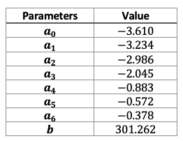
Table 1. Fitted parameters in demand forecast model

The parameters for price optimization are defined in Table 2. The objective is to optimize the next n=7 days’ price to maximize the total revenue of the next 7 days. There are m=7 price options for each day. Thus, the actual solution space contains a total of mⁿ= 823,543 candidates. Therefore, a total of mn=49 unique binary variables [x_T, … , x_T+6] are defined in the objective function, which incorporates total revenue, prediction uncertainty, and penalty of equality constraints for ensuring prices to be selected within available price options. Overall, this setup results in a QUBO search space with 2⁴⁹= 5.6 ×10¹⁴ possible solutions.

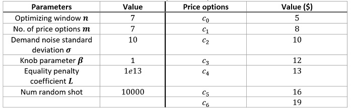
Table 2. Optimization parameters

Once our problem is set up, it only takes a few seconds to run 10,000 shots and return the optimized results. The single lowest cost/energy among these 10,000 shots is -12752.164, representing the objective function H. For comparison, to assess the quality of the result, we also iterate (by brute-force) through the whole solution space, i.e. all the 7⁷=823,543 possible price configurations, to obtain the energy for each one, which takes more than 5 minutes to run on a standard ml.m5.2xlarge AWS instance. We plot the distribution of these energy values of the whole solution space as shown in Figure 1, where the red line is plotted to show the single lowest energy value obtained from the quantum annealer in our 10,000 shots . We can see that the value (-12752.164) from the quantum annealer is close to the ground global minimum (-12802.802).

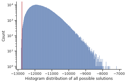
Figure 1. Result Quality

We can decode the response into actual price results, as shown here. The optimized price path is [19, 12, 12, 10, 19, 10, 16].

def decoder_price_response(response, n_days, price_options):
”””
    Args:
    Response: the response from Amazon Braket
    n_days (int): the number of days for optimizing prices
	price_options (list): the list of price choices each day
Return:
	opt_decoded_prices (list): the optimized price values
	opt_prices (np.array): the binary encoded optimized prices
	energy: the value energy, i.e. objective function 
”””
    opt_price, energy = response.record.sample[response.record.energy.argmin()], response.record.energy.min()
    prices = []
    for i in range(n_days):
        price_i = opt_price[i*len(price_options): (i+1)*len(price_options)]
        assert price_i.sum()==1
        prices.append(price_options[price_i.argmax()])
    return prices, opt_price, energy

opt_decoded_prices, opt_prices, energy =decoder_price_response(response, len(a), price_levels)
opt_decoded_prices, opt_prices, energy

([19, 12, 12, 10, 19, 10, 16],
 array([0, 0, 0, 0, 0, 0, 1, 0, 0, 0, 1, 0, 0, 0, 0, 0, 0, 1, 0, 0, 0, 0,
        0, 1, 0, 0, 0, 0, 0, 0, 0, 0, 0, 0, 1, 0, 0, 1, 0, 0, 0, 0, 0, 0,
        0, 0, 0, 1, 0], dtype=int8),
 -12752.164)

Trade-off between maximizing revenue and minimizing risk

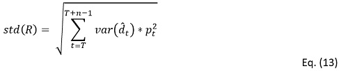
In order to investigate the trade-off between the expected revenue and prediction uncertainties, we vary the Knob parameter β within a large range of [10², 10⁹] and run multiple experiments on D-Wave with different β values. The results are shown in Figure 2, where each dot represents the optimized result with the lowest energy value of an experiment with x-axis representing its expected revenue and y-axis representing the estimated standard deviation of revenue std(R). The standard deviation of revenue can be derived from the estimated variance of the predicted demand:

The red line shows the Pareto front, where the expected revenue will increase together with the increase of the standard deviation (i.e. uncertainties), and the other way around.

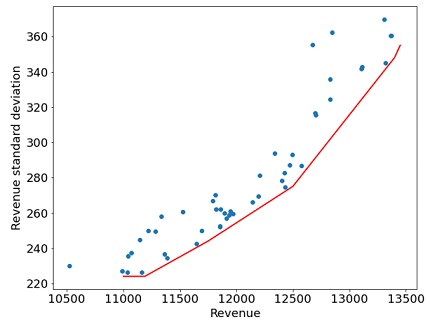
Figure 2. Pareto front for trade-off between expected revenue and prediction variance

We see that the expected revenue can vary significantly between 10,000 and 13,500, while the estimated standard deviation of the revenue (i.e., uncertainty) can change in a large range [200, 380] as well. The figure shows that as the expected revenue increases, the estimated standard deviation of the revenue will also increase. This means that if we select a price solution for higher expected revenue, the uncertainties will increase at the same time. This is due to the fact that the demand estimation model will become less confident about its predictions with a price configuration of high expected revenue. This observation illustrates that there is a trade-off between maximizing the revenue and minimizing the uncertainty. High revenue and rewards usually accompany high uncertainty and risk. In practice, according to different business strategies and needs, we usually need to find an appropriate 𝛽 to maximize the revenue under an acceptable level of uncertainty.

Conclusion

In this blog, we demonstrated how a quantum annealer on Amazon Braket can be used to solve a price optimization use case. We showed how to mathematically formulate the problem within the quantum-ready QUBO framework, and then we subsequently ran the optimization problem on a D-Wave quantum annealer. By using this type of approach, customers can explore the current capabilities of quantum hardware and plan how they could use Amazon Braket to help tackle combinatorial optimization challenges to assist their business and operations decisions.

Reference

[1] Glover, F., Kochenberger, G. and Du, Y., 2019. Quantum Bridge Analytics I: a tutorial on formulating and using QUBO models. 4OR, 17(4), pp.335-371.

[2] Kochenberger, G., Hao, J.K., Glover, F., Lewis, M., Lü, Z., Wang, H. and Wang, Y., 2014. The unconstrained binary quadratic programming problem: a survey. Journal of combinatorial optimization, 28(1), pp.58-81.

[3] Anthony, M., Boros, E., Crama, Y. and Gruber, A., 2017. Quadratic reformulations of nonlinear binary optimization problems. Mathematical Programming, 162(1), pp.115-144.

[4] Cruz-Santos, W., Venegas-Andraca, S.E. and Lanzagorta, M., 2019. A QUBo formulation of Minimum Multicut problem instances in trees for D-Wave Quantum Annealers. Scientific reports, 9(1), pp.1-12.

[5] Ben-Tal, A. and Nemirovski, A., 2002. Robust optimization–methodology and applications. Mathematical programming, 92(3), pp.453-480.

[6] Fabozzi, F.J., Kolm, P.N., Pachamanova, D.A. and Focardi, S.M., 2007. Robust portfolio optimization and management. John Wiley & Sons.

[7] Zaman, M., Tanahashi, K. and Tanaka, S., 2021. PyQUBO: Python library for mapping combinatorial optimization problems to QUBO form. arXiv preprint arXiv:2103.01708.

AWS Quantum Technologies Blog

Using quantum annealing on Amazon Braket for price optimization

QUBO basics

Overall objective function

The Expected Revenue

Prediction Uncertainty

Incorporate equality constraints

Minimizing QUBOs on Amazon Braket

Amazon Braket for QUBO problems

How to solve QUBOs on Amazon Braket

Train demand forecast model

Construct and solve QUBO on Amazon Braket

Experiment Results

Trade-off between maximizing revenue and minimizing risk

Conclusion

Reference