How to use pulse-level control on OQC’s superconducting quantum computer

This post was contributed by Jamie Friel and Bryn Bell from Oxford Quantum Circuits (OQC), and Jordan Sullivan from the Amazon Braket team in AWS.

Amazon Braket Pulse enables users to control and modify the low-level analog instructions for quantum computers, to optimize performance or develop new analog protocols, like error suppression and mitigation.

The use of predefined quantum gates is a common approach to perform operations on a quantum computer. However, this approach can be limiting for users who wish to investigate noise characteristics of particular quantum devices or test quantum error mitigation techniques, as these applications require lower-level control of the device, typically called “pulse-level control.”

Users of Amazon Braket and OQC’s private cloud have pulse-level access to OQC’s superconducting quantum device. This provides them the ability to precisely control gate calibration and gain a finer-grained view on fidelity metrics and system characterization. Pulse control on Amazon Braket is based on the open-source OpenPulse library and currently extends to multiple quantum devices on the service in addition to OQC.

In this post, we’ll highlight the power of pulse control in more detail by providing several demonstrations of use cases that it unlocks on the OQC device, down to the level of fundamental quantum physics. Along the way we’ll explain some best practices to get the most out of these devices.

Pulse-level control in the hands of our users

Normally, when you submit a gate-based quantum program to OQC via Amazon Braket, OQC compilers translate the gates into analog pulses, since all quantum computers are indeed controlled with analog signals at the lowest level. In the case of OQC’s superconducting quantum devices, these are microwave pulses. However, users can now bypass the compilation step and directly implement quantum operations with pulse-parameter precision. It enables them to define key characteristics such as: frequency, phase, amplitude, pulse duration, and pulse shape.

What are pulse frames?

A key object within the Braket Pulse library is the Frame. A frame contains a series of pulses which can be sent to or received back from the quantum computer, for example, to address a qubit transition, like flipping the state from |0> to |1>. To manipulate pulses in a frame, we specify parameters such as pulse amplitude and duration, with which a wide array of experiments can be performed. Frame types are device-specific. To help you getting started, Braket Pulse provides a set of predefined frames which are included for OQC’s device:

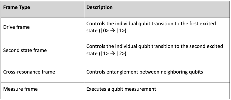
Table 1: Types of Frame in Braket Pulse

We will next give several examples of how these parameters can be used to enable new capabilities of OQC’s quantum hardware. We will focus on three demonstrations covering coherence metrics, single-qubit gate calibration, and cross-resonance characterization. Drive and cross-resonance frames will play a crucial role in the following examples with Braket Pulse.

Demo 1 – Coherence Metrics

One of the key metrics of qubit quality is coherence time – the length of time a qubit can store a quantum state before it loses its quantum properties due to interaction with the environment. Before we manipulate a qubit, we must characterize its coherence time to know how long we can interact with it. One measure of qubit coherence is its energy relaxation time, otherwise known as ‘T₁’. T₁ is a measure of the lifetime of a qubit in the excited state, before it decays to the ground state.

To characterize T₁ we first prepare the qubit in the excited state by applying an x gate. We then wait for a specific time (delay duration) and measure whether the qubit is still in the excited state. By varying the delay time, we can trace out an exponential decay of the excited state population, and extract the T₁ time constant. The code below demonstrates these steps on Amazon Braket. Note how with Braket Pulse we can mix and match gates (an x gate here) with pulses (the delay τ) in the same program.

from braket.aws import AwsDevice
from braket.circuits import Circuit, FreeParameter
from braket.pulse import PulseSequence, ConstantWaveform
import numpy as np

N_shots = 100
device = AwsDevice(“arn:aws:braket:eu-west-2::device/qpu/oqc/Lucy”)

def generate_circuit_t1(qubit: int) -> Circuit:
    drive_frame = device.frames[f”q{qubit}_drive”]

    delay_pulse = ( 
        PulseSequence()
        .delay(drive_frame, FreeParameter(“tau”))
    )
    
    # Generate a circuit that performs an X rotation and then adds a delay
    return Circuit().x(qubit).pulse_gate(qubit, delay_pulse) 

# Create an array of delays, from 0s to 80us
delays_t1 = np.linspace(start_delay_t1:=0, end_delay_t1:=80e-6, 50)

circuit_template_t1 = generate_circuit_t1(qubit=5)
circuits_t1 = [circuit_template_t1(tau=delay) for delay in delays_t1]
batch_t1 = device.run_batch(circuits_t1, shots=N_shots)

Figure 1 shows the result of such a program. We model the T₁ time by fitting an exponential decay exp(-t/T₁). We can derive a value of ~23us for T₁, highlighted as a red line in Figure 1. By understanding the decay time constant, T₁, a user can better estimate whether energy relaxation may be a dominating source of errors in a computation. It is important to keep in mind that quantum computers are highly sensitive to noise, which can cause errors impacting the quality of the output. The better we understand these sources of error, the better we can mitigate them to achieve higher quality results.

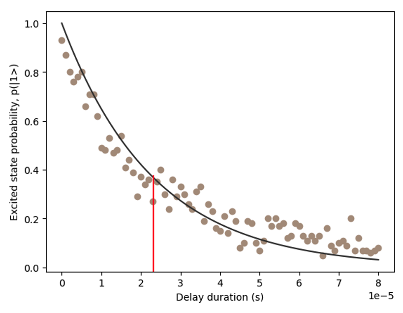
Figure 1 – Change in probability of excited state p(|1>) with increasing delay duration. The red line highlights the derived T1 time of ~23us.

OQC provides regular updates of coherence times in the Braket device details page. In the next section of this post, we will demonstrate how users can investigate these metrics directly and at a deeper level. This enables researchers to investigate and characterize device-specific noise, understand how it affects qubits in a computation, and develop new protocols to counteract the impacts of noise, for instance: error mitigation and noise-adaptive compilation techniques.

Demo 2 – Single-qubit calibration

Next, we demonstrate how users can manipulate an individual qubit’s state. This means we will highlight how a qubit can be controlled between its ground state and first excited state, at the pulse level. To achieve this, energy must be added to the system. We can do so by ‘injecting’ microwave control pulses of a specific duration and frequency.

The code below demonstrates how to use a drive frame to define such a microwave pulse-duration to control a qubit.

def generate_drive_sequence(qubit: int, amplitude: float=0.03) -> PulseSequence:
    readout_frame = device.frames[f"r{qubit}_measure"]
    drive_frame = device.frames[f"q{qubit}_drive"]
 
    length = FreeParameter("length")
    constant_drive_wave = ConstantWaveform(length, amplitude)
    
    # Generate drive pulse of given duration and measure
    # Default pulse is a constant shaped pulse of amplitude 0.03
    # This is approximately where Lucy's single qubit gates are calibrated
    return ( 
        PulseSequence()
        .play(drive_frame, constant_drive_wave)
        .capture_v0(readout_frame)
    )

drive_lengths = np.linspace(drive_start:=8e-9, drive_end:=1e-6, 50)

drive_pulse_template = generate_drive_sequence(qubit=2)
drive_pulse_sequences = [drive_pulse_template(length=pulse_length) for pulse_length in drive_lengths]

drive_pulse_batch = device.run_batch(drive_pulse_sequences, shots=N_shots)

Running this code gives us the results shown in Figure 2.

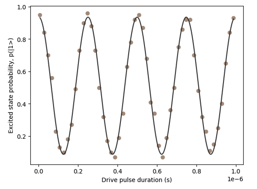
Figure 2 – Excited state probability as a function of pulse duration.

Figure 2 shows the characteristic sinusoidal form of a Rabi oscillation representing how the qubit rotates between its ground and excited state. By measuring this oscillation rate, we can determine a precise pulse-duration for a given qubit rotation angle (i.e., how long we need to drive the qubit with our microwave pulses to get it to transition from |0> to |1>) and therefore ensure a low-error single qubit gate.

A high-quality single qubit gate also requires that the microwave pulse frequency is precisely matched to the qubit’s transition frequency. Braket Pulse allows users to manipulate the frequency with which they drive the qubit. Let’s see what happens if we detune our frame (i.e., changing the frequency from the default value) by a small amount and perform the same drive pulse over time, applying the code below:

def generate_rabi_spectroscopy_sequence(qubit: int, amplitude:float=0.03) -> PulseSequence:
    readout_frame = device.frames[f"r{qubit}_measure"]
    drive_frame = device.frames[f"q{qubit}_drive"]
    
    length = FreeParameter("length")
    frequency_detune = FreeParameter("frequency_detune")
    rabi_drive_waveform = ConstantWaveform(length, amplitude)
    
    # Detune the frequency using the set_frequency method
    # subtracting the detuning from the current frame frequency
    rabi_sequence = ( 
        PulseSequence()
        .shift_frequency(drive_frame, -frequency_detune)
        .play(drive_frame, rabi_drive_waveform)
        .capture_v0(readout_frame)
    )
    return rabi_sequence
# Array of driving pulse length. Minimum pulse length on Lucy is 8ns, so we do not start at 0s
lengths_rabi = np.linspace(start_rabi:=8e-9, end_rabi:=2.5e-6, 50)
# Detuning array of 500mhz
# Lucy's frequencies will typically be 4-5ghz, so this is a broad range in terms of an individual qubit
detune_lengths = np.linspace(detune_end:=-1.5e7, detune_start:=1.5e7, 50)

rabi_pulse_template = generate_rabi_spectroscopy_sequence(qubit=5)
batches_rabi_spectroscopy = []
for detune in detune_lengths:
    rabi_pulse_sequences = [rabi_pulse_template(length=pulse_length, frequency_detune=detune) for pulse_length in lengths_rabi]
    detune_batch = device.run_batch(rabi_pulse_sequences, shots=N_shots)
    batches_rabi_spectroscopy.append(detune_batch)

Running this code results in the data in Figure 3, representing the characteristic ‘chevron’ pattern that is produced when driving a qubit. The oscillation contrast is highest and oscillation rate lowest when the drive frame is precisely resonant with the qubit frequency transition. Like in Figure 3, when calibrated, this resonance should occur at 0 Hz frequency detuning. Therefore, such a measurement can tell us how well we’ve calibrated the drive frame of our qubit control operations.

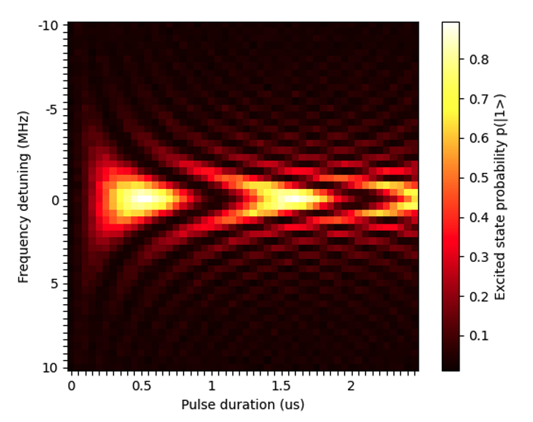
Figure 3 – Depicts a heat map of the excited state probability as it varies with pulse duration and frequency detuning. The oscillation contrast is highest and oscillation rate lowest when the drive frame is precisely resonant with the qubit frequency transition. When calibrated, this resonance should occur at 0 Hz frequency detuning.

Further applications for low-level quantum device calibration

Low-level device calibration can help improve performance in several different ways. We can use it to improve gate performance using error mitigation techniques, like in Zero Noise Extrapolation, where we perform quantum operations with a range of noise levels and extrapolate the results to a hypothetical “zero noise” scenario. Another application is tracking the robustness of gate calibration procedures in real time during a quantum computation.

Demonstration 3 – Cross-resonance characterization

Having covered the manipulation of a single qubit, we now demonstrate how users can control the entanglement of multiple qubits.

There are several methodologies for entangling qubits. In the OQC system, qubits are entangled through a ‘cross-resonance’ microwave pulse. In such an entangling gate, a microwave pulse is applied to the physical control port of one qubit, but at a frequency which is resonant with another qubit. This generates a driving effect on the second qubit like the Rabi oscillation, but at a rate crucially dependent on the state of the first qubit. More information on the calibration of cross-resonant gates on a Coaxmon, OQC’s patented qubit architecture, can be found in Patterson, A.D., et al. (2019), Calibration of the cross-resonance two-qubit gate between directly-coupled transmons, Phys. Rev. Applied 12, 064013.

Putting this into practice, we can observe the dynamics of this gate with Braket Pulse. To do this, we prepare qubit #4 (otherwise known as the ‘control’ qubit) in its excited |1> state. We then modify the pulse in the cross-resonance frame that acts on the control qubit. By increasing the drive pulse duration, we can measure its effect on the ‘target’ qubit #5. We then repeat this process but with both qubits beginning in their ground |0> state.

def generate_cross_resonance_circuit(edge:tuple[int,int], initial_state:int) -> Circuit:
    control_qubit, target_qubit = edge

    drive_frame = device.frames[f"q{control_qubit}_q{target_qubit}_cross_resonance"]
    cancel_frame = device.frames[f"q{control_qubit}_q{target_qubit}_cross_resonance_cancellation"]

    duration = FreeParameter("duration")
    
    cross_res_waveform = ConstantWaveform(length=duration, iq=cross_res_amps[edge])
    const_cancel = ConstantWaveform(length=duration, iq=cross_res_cancelations_amps[edge])

    cross_res = ( 
        PulseSequence()
        .play(drive_frame, cross_res_waveform)
        .play(cancel_frame, const_cancel)
    )

    circuit = Circuit().x(control_qubit) if initial_state == 1 else Circuit()
    return circuit.pulse_gate(edge, cross_res)

# Crossresonant gates take a much longer time than one-qubit gates
# As such we increase the time to 1400ns
durations = np.arange(start_cross_res:=8e-9, end_cross_res:=1400e-9, 75e-9)

pulse_sequences_cross_res = {}
batch_cross_res = {}
for initial_state in [0,1]:
    circuit = generate_cross_resonance_circuit(edge=(4,5), initial_state=initial_state)
    pulse_sequences_cross_res[initial_state] = [circuit(duration=duration) for duration in durations]
    batch_cross_res[initial_state] = device.run_batch(pulse_sequences_cross_res[initial_state], shots=N_shots)

The results of this experiment are shown in Figure 4 and demonstrate the dynamics of a target qubit when the control qubit is initially in state |0> (blue dots) or |1> (orange dots) during a cross-resonance pulse.

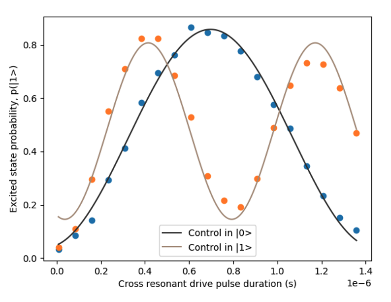
Figure 4 – The dynamics of the cross resonant gate with increasing pulse duration.

Figure 4 shows the excited state probability of the target qubit after the control qubit has been driven by a cross resonant pulse for a given time length. In the case where the control qubit was in state |1>, the target qubit has returned to its original state (considering some allowance for noise). Conversely, when the control qubit was in state |0>, the target qubit ends up in a different state. We fitted two sine curves to the data generated in Figure 4 which shows up as two Rabi oscillations of different frequencies, like Figure 2.

Here we have demonstrated the core behavior of an entangling gate and a building block for the gates that we use at OQC to generate entanglement. Controlling the pulse duration, amplitude, and frequency all play a critical role in the calibration of two-qubit gates which can now be investigated using OpenPulse on OQC’s quantum computer. For instance, increasing the amplitude will lead to an overall faster two-qubit gate, at the cost of more errors. Finding this balance is key to stable and accurate calibration of the OQC device.

Further applications for novel gate designs

By incorporating pulse control techniques, we can significantly enhance the performance of cross-resonance gates compared to their abstract gate counterparts. Moreover, leveraging the power of TensorFlow can enable us to optimize gate design under complex constraints. This opens opportunities for fine-tuning and refining gate operations. We can even implement quantum optimal control to allow for more efficient and precise qubit manipulations. Lastly, optimization of pulses presents a promising avenue to further improve gate design by continuously refining and optimizing the applied pulses.

Conclusion

In this post, we have gone over some of the fundamental components of quantum computation at the pulse level. We looked at how the coherence metrics can be measured, how we can calibrate single-qubit gates, and how we characterize cross-resonance driving.

These are the core components of any quantum program running on OQC’s quantum hardware. This same pulse-level control is fully available for you to explore, thanks to Amazon Braket Pulse.

We’re excited for you to experiment with this low-level control on OQC’s quantum computing hardware by using one of the available pulse example notebooks!

AWS Quantum Technologies Blog