AWS Quantum Technologies Blog
Suppressing errors with dynamical decoupling using pulse control on Amazon Braket
Introduction
The quantum state of a qubit is extremely fragile, as any interaction with its environment generally results in uncontrolled changes. The fragility of quantum states means that errors are a fundamental problem for quantum computers, making quantum error correction a key enabler for using quantum computing to solve large problems. However, error correction is itself an error-prone process. In order to be successful, an error correction protocol must correct more errors than it introduces, which requires the baseline level of error in a quantum computer to drop below a certain level, also called the error threshold. An indispensable precursor to error correction is therefore quantum error suppression, which refers to a variety of techniques that effectively reduce the baseline level of error in a quantum computer.
In this blog post, we introduce and demonstrate an error suppression technique known as dynamical decoupling, which can significantly extend the lifetime of qubits during a quantum computation. We start with an introduction to dynamical decoupling, and provide an example of how pulse control on Amazon Braket enables the low-level control that is required to execute dynamical decoupling protocols on current quantum hardware. The Python code in this blog is taken from the Amazon Braket module of SuperstaQ, Super.tech’s write-once-target-all platform for optimizing application performance by tailoring a quantum program to a desired piece of quantum hardware. You can reproduce the results in this blog by downloading the notebook that demonstrates dynamical decoupling using Braket here, as well as the supporting SuperstaQ module here.
Dynamical Decoupling and the Spin Echo
The state of a qubit in isolation can be represented by a point on the Bloch sphere (see Figure 1 below), on which the north and south poles correspond, respectively, to 0 and 1 states. Points on the equator correspond to superpositions of 0 and 1 in which the qubit is equally likely to be found in the state 0 or 1 upon measurement. Undesired physical processes in a quantum computer can lead to a variety of qubit errors, such as relaxation errors, whereby a qubit “gravitates” toward to the 0 state by losing energy to its environment, and dephasing errors, whereby a stray photon bounces off of the qubit, causing the qubit to spin around the Bloch sphere and change its latitude by an unknown angle. These processes destroy the quantum information stored in a qubit.
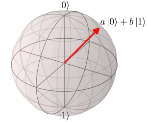
Figure 1 Unlike a classical bit, which can only be in the state 0 or 1, a qubit can be in a superposition of 0 and 1, represented by a point on the surface of a sphere, and mathematically written as a|0> + b|1>.
Since relaxation and dephasing errors are the result of an interaction between a qubit and its environment, we can mitigate these errors by trying to actively (or dynamically) undo the effects of this interaction (which physicists call a coupling) – that is, we can perform dynamical decoupling.
Generally speaking, any interaction between a qubit and its environment can be represented with a rotation of the qubit state around the Bloch sphere. Different states of the environment will cause the qubit to rotate in different directions and by different amounts (see Figure 2 below). However, we can mitigate environmental errors with a protocol that causes these rotations to cancel themselves out.
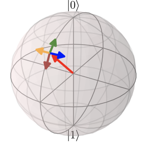
Figure 2 The environment can cause the qubit to rotate in different directions, represented by small arrows pointing away from an initial state of the qubit. The basic strategy for dynamical decoupling is to undo any rotation caused by the environment, regardless of which rotation actually occurs.
Consider a simplified example where the environment has only two possible states: a state |↻> that causes the qubit to rotate clockwise around the Z axis running from the north pole to the south pole, and a state |↺> that causes the qubit to rotate in the opposite direction (counterclockwise) around the same axis. Since the actual state of the environment is unknown, if we initialize a qubit to a point on the equator, after some time we will not know which way the qubit has rotated – the qubit has experienced dephasing. However, we can undo this dephasing with a trick visualized in Figure 3 below: we can use an electromagnetic pulse, called a π pulse (pronounced “pie pulse”), to quickly rotate the qubit by 180° around an axis in the equator. If the environment was in the “clockwise” state |↻>, the qubit will now be at a point located counterclockwise from its original location. Letting the qubit continue to interact with the environment will then bring the qubit back to its original state [1]. Crucially – the qubit comes back to its original state even if the environment was actually in the “counterclockwise” state |↺>! This trick, invented by Erwin Hahn in 1950 [2], is known as the spin echo, and is the first dynamical decoupling sequence. Spin echoes are used daily for magnetic resonance imaging (MRI) in hospitals to extract images that otherwise get blurred out by the dephasing of the nuclear spins of atoms in biological tissue [3].
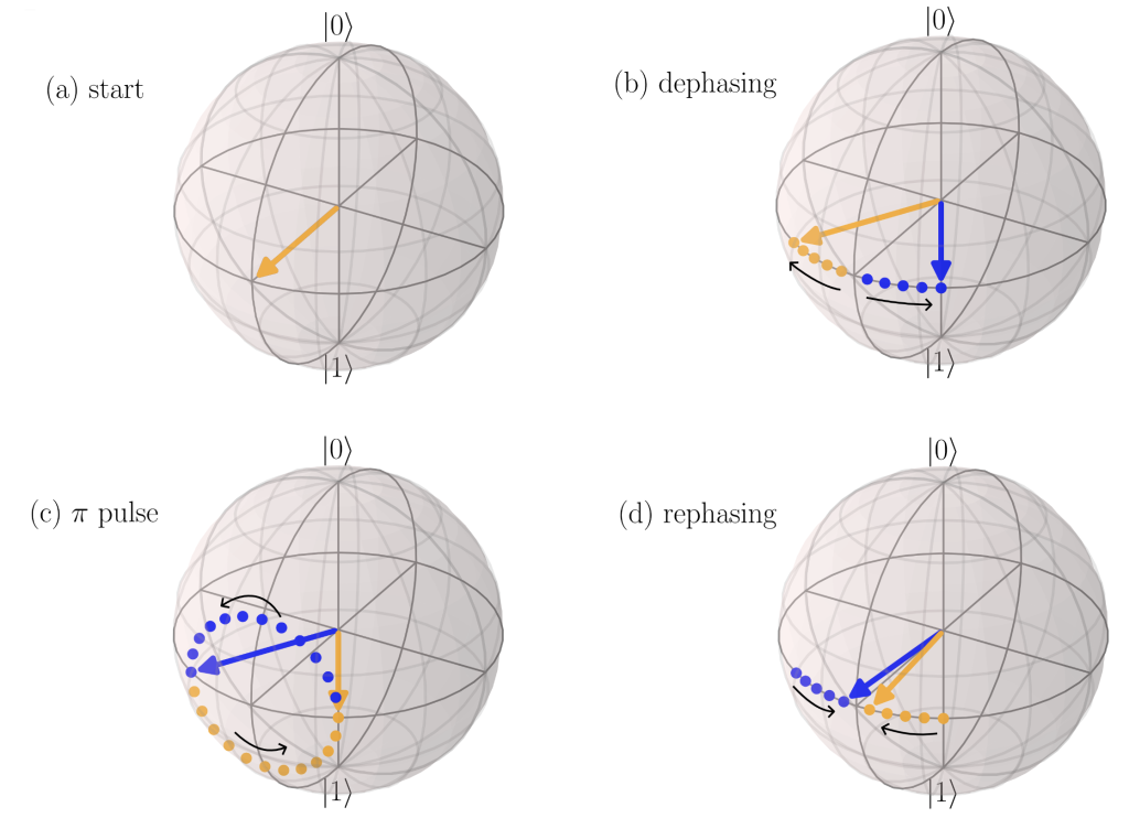
Figure 3 Visualization of the spin echo. (a) A qubit is initialized to a state on the equator. (b) Interacting with its environment initially causes a qubit to dephase by rotating in an unknown direction; two possibilities are here represented by blue and orange arrows. (c) After some dephasing, a rapid π pulse rotates the qubit by 180° around an axis in the equator [1], after which (d) continued interaction with the environment causes the qubit to “rephase” and return to its original state. The amount of dephasing that occurs during the π pulse is negligibly small if this pulse is fast compared to the rate of dephasing. You can download an animated visualization of the spin echo here.
Carr-Purcell-Meiboom-Gill and XY Sequences
While the spin echo is sufficient to prevent dephasing caused by a static environment, changes to the environment may result in changes to the speed at which a qubit rotates, preventing the rotations before and after the spin echo π pulse from cancelling out. To fix this problem, a dynamical decoupling protocol known as the Carr-Purcell-Meiboom-Gill (CPMG) sequence [4, 5] puts a rapid spin echo on repeat: (1) wait for a short time τ, (2) apply a π pulse around a fixed axis in the equator, (3) wait for the same time τ, and (4) repeat from step 1. As long as the time τ is small compared to the time scale on which the environment changes significantly, the qubit will rotate in opposite directions by approximately equal amounts between consecutive pairs of π pulses, causing these rotations due to environmental effects to cancel out.
CPMG is excellent at preventing dephasing errors, but there are other errors that it cannot prevent. For example, CPMG does not protect against unwanted rotations around the same axis as the CPMG π pulses. Fortunately, this shortcoming can be fixed by using different axes of rotation for different π pulses. Universal dynamical decoupling sequences – that is, sequences that protect against all types of unwanted rotations – are therefore typically defined by a choice of when to apply π pulses, and which axes to use for these pulses. These choices are where the pulse-level control provided by Amazon Braket will come into play for running dynamical decoupling sequences!
The simplest universal dynamical decoupling sequence applies a sequence of equally-spaced π pulses much like CPMG, but alternates the axis of rotation for these π pulses between two axes spaced 90° apart on the equator. These rotation axes are commonly referred to as the X and Y axes. One “cycle” of this sequence, aptly known as the XY4 sequence, consists of four pulses visualized in Figure 4 below. As it turns out, all four pulses are necessary to bring an arbitrary qubit state on the Bloch sphere back to its original location, so the XY4 sequence repeats the entire four-pulse cycle.
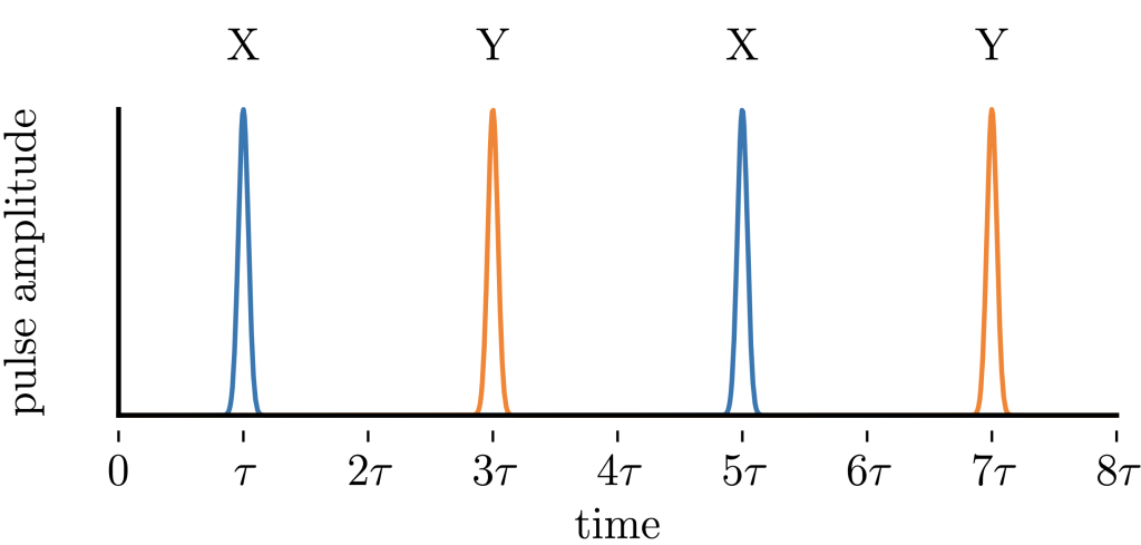
Figure 4 A single cycle of the XY4 dynamical decoupling sequence. This cycle can be repeated many times to suppress errors that would otherwise accumulate while a qubit is idle.
While there are many more sophisticated dynamical decoupling sequences [6], generally involving unevenly spaced pulses with judiciously chosen pulse axes (all of which can be chosen with Amazon Braket), to keep things simple we will stick to the XY4 sequence. However, it is worth noting that even relatively minor modifications to CPMG and XY4 make these sequences competitive with the state-of-the-art methods for dynamical decoupling [6].
Constructing a Dynamical Decoupling Sequence with Braket Pulse
We now show dynamical decoupling in action, enabled by the pulse-level control and timing capabilities provided by Amazon Braket. To this end, our fundamental building block is a “delay” or “idle” instruction that can be used to control the timing between different pulses in a dynamical decoupling sequence. We can construct an idle instruction (or an idle gate) using the PulseSequence object as follows:
from braket.aws import AwsDevice
from braket.pulse import PulseSequence
from braket.circuits import Circuit

device = AwsDevice("arn:aws:braket:us-west-1::device/qpu/rigetti/Aspen-M-2")

def idle_gate(qubit, idle_time):
    """
    Return an "idle" gate that enforces a delay between consecutive instructions that address the given qubit.
    """
    control_frame = device.frames[f"q{qubit}_rf_frame"]
    pulse_sequence = PulseSequence().delay(control_frame, idle_time)
    return Circuit().pulse_gate(qubit, pulse_sequence)
Note that defining pulse-level instructions generally requires choosing a specific quantum processor (or a specific device; we chose Rigetti’s Aspen M2 QPU), as well as a control frame for the qubits addressed by the instruction. You can learn more about pulse sequences and control frames in another blog post here.
The idle gate allows us to construct an XY4 dynamical decoupling sequence, which protects a qubit from errors that accumulate when it would otherwise be idle:
def idle_with_XY4(qubit, idle_time, num_cycles):
    """
    Construct an XY4 pulse sequence with a fixed number of cycles and a total duration 'idle_time' for a given qubit.
    """
    total_pulse_number = 4 * num_cycles                        # there are four pi pulses per XY4 cycle
    pulse_spacing = idle_time / total_pulse_number             # the delay time between consecutive pulses (namely, 2 tau)
    pulse_padding = idle_gate(qubit, pulse_spacing / 2)        # each pulse gets padded by half of the delay time between pulses
    padded_x = pulse_padding + x_pulse(qubit) + pulse_padding  # padded X pulse
    padded_y = pulse_padding + y_pulse(qubit) + pulse_padding  # padded Y pulse
    cycle = [padded_x, padded_y, padded_x, padded_y]           # a single XY4 cycle
    return Circuit(cycle * num_cycles)                         # a cirucit of 'num_cycles' XY4 cycles
Here x_pulse is a 180° rotation around the X axis (more details can be found in the Braket SuperstaQ module here), while padded_x is an instruction that inserts the entire intervals from 0 to 2τ and 4τ to 6τ in Figure 4 above. Similarly, y_pulse is a 180° rotation around the Y axis, and padded_y corresponds to the intervals from 2τ to 4τ and 6τ to 8τ in Figure 4.
Demonstration on a Rigetti QPU
Now that we have constructed a dynamical decoupling sequence, we are ready to demonstrate its benefits on a quantum processor. To this end, we run a simple experiment: initialize a qubit in the 1 state, and watch it “relax” to 0, both with and without the use of dynamical decoupling to suppress relaxation errors. This experiment is defined by two circuits that are described as follows:
import braket_superstaq_demo as bss

def relax_with_idle(qubit, idle_time):
    """
    Flip a qubit from |0> to |1>, and let it idle for a given time.
    """
    return bss.x_pulse(qubit) + bss.idle_gate(qubit, idle_time)


def relax_with_XY4(qubit, idle_time, num_cycles):
    """
    Flip a qubit from |0> to |1>, and run an XY4 sequence with a fixed number of cycles and total duration.
    """
    return bss.x_pulse(qubit) + bss.idle_with_XY4(qubit, idle_time, num_cycles)
Since the quantum processor we are using starts with all qubits in their 0 state, in the first circuit we first apply an initial π pulse to move the target qubit to the 1 state, and then let the qubit idle for a variable amount of time. In the second circuit, we insert an XY4 sequence during the idle time.
We now choose different idling times, and for each time we estimate the probability that the qubit is still in the 1 state at the end:
import numpy as np

def probability_of_1(circuit, shots):
    """Run a single-qubit circuit and return the probability of measuring the qubit in the 1 state."""
    task = bss.device.run(circuit, shots=shots)
    return task.result().measurement_counts["1"] / shots

qubit = 4  # qubits are identified by an integer index
shots = 1000  # number of times to run a circuit in order to estimate probabilities of different outcomes
idle_times = np.arange(2, 61, 2) * 1e-6  # 2, 4, 6, ..., 60 microseconds
decoupling_cycles = 2  # number of XY4 cycles

relaxation_fidelities_with_idle = [
    probability_of_1(
        relax_with_idle(qubit, idle_time),
        shots=shots,
    )
    for idle_time in idle_times
]

relaxation_fidelities_with_XY4 = [
    probability_of_1(
        relax_with_XY4(qubit, idle_time, num_cycles=decoupling_cycles),
        shots=shots,
    )
    for idle_time in idle_times
]
Here shots is the number of times that we run a given circuit to estimate the probability of measuring 0 or 1. We made a few arbitrary choices for this experiment concerning which qubit to use, the number of shots, the idle times to inspect, and the number of XY4 cycles – we encourage you to try out different values in the notebook for yourself!
The results from running the above code are as follows, shown in Figure 5 below:
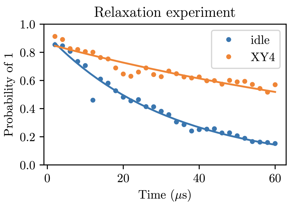
Figure 5 Probability of measuring a qubit in the 1 state after a qubit relaxation experiment, which consists of initializing the qubit in 1, and subsequently either letting the qubit idle or running an XY4 dynamical decoupling sequence. Lines show a fit to exponential decay.
Here each data point correspond to an experimental outcome, and an exponential decay curve P (|1>)= e– t/T1 is used to fit the results of both experiments. In the formula of the fitting curve, T1 can be interpreted as a “lifetime” of the |1> state, which our experiment finds is about 30 microseconds for an idling qubit. If we insert an XY4 sequence with only 2 cycles, i.e. 8 π pulses, this lifetime gets by a factor of 4!
However, merely extending the lifetime of the 1 state is not enough to have a qubit that is truly “quantum”, and distinct from a classical bit that has an unknown probability of being in 0 or 1. A qubit must also preserve its coherence, the information about its longitudinal position on the Bloch sphere. To demonstrate the preservation of coherence, we can use a π/2 pulse (that is, a 90° rotation) to rotate a qubit that is initially in the 0 state into a location on the equator, let the qubit idle (or insert a dynamical decoupling sequence), then rotate back to 0 by undoing the original π/2 pulse:
def check_coherence_with_idle(qubit, idle_time):
    """
    Rotate a qubit from |0> to the equator, let it idle, and rotate it back.
    """
    return (
        bss.x_pulse(qubit, angle=np.pi / 2)
        + bss.idle_gate(qubit, idle_time)
        + bss.x_pulse(qubit, angle=-np.pi / 2)
    )

def check_coherence_with_XY4(qubit, idle_time, num_cycles):
    """
    Rotate a qubit from |0> to the equator, let it "idle" with dynamical decoupling, and rotate it back.
    """
    return (
        bss.x_pulse(qubit, angle=np.pi/2)
        + bss.idle_with_XY4(qubit, idle_time, num_cycles)
        + bss.x_pulse(qubit, angle=-np.pi/2)
Just as in the previous experiment, we now choose different idling times, but this time examine the probability that the qubit ends up in 0. The results are in Figure 6:
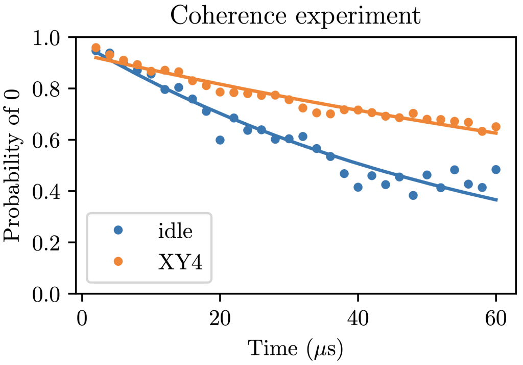
Figure 6 Probability of measuring a qubit in the 0 state after running a quantum coherence preservation experiment, which consists of (1) rotating the qubit from 0 to a state on the equator, (2) either letting the qubit idle or running an XY4 dynamical decoupling sequence, and (3) undoing the initial rotation. Lines are provided purely as a guide to the eye, since this probability should approach 0.5 as the qubit completely loses its quantum coherence.
The lines in Figure 6 above are again a fit to a simple exponential decay curve, but note that the corresponding decay rate can no longer be cleanly interpreted as a “coherence time”, since there are several concurrent phenomena that affect the results in Figure 6 [7]. Even so, we clearly see that inserting a 2-cycle XY4 sequence has increased the coherence time of the qubit by roughly a factor of 2!
Conclusion
In order to suppress errors in today’s quantum computers, researchers require low-level access to quantum devices. In this blog post, we have provided a pedagogical tutorial to dynamical decoupling, a pulse-level technique for suppressing the baseline level of error in a quantum computer. Starting with the spin echo, we built up to CPMG, and finally XY4, the simplest sequence that is in principle capable of suppressing any qubit idling error. We showed an example of how SuperstaQ uses the newly released pulse-level control on Amazon Braket to construct dynamical decoupling sequences, and demonstrated that these sequences increase the lifetime of a qubit. These sequences can be inserted into any location in a circuit when a qubit would otherwise be idle, and thereby suppress errors that would build up on idling qubits.
To experiment with dynamical decoupling and boost the performance in your own quantum circuits, you can download the notebook used in this blog post here, and the supporting python module here. For practitioners interested in a deeper dive, there is a broad family of sophisticated dynamical decoupling sequences and compilation strategies that further enhance error suppression techniques [6]. To learn more about what dynamical decoupling can accomplish, you can take a look at these recent articles [6, 8, 9, 10], and start using pulse-level control to boost your quantum program performance today.
References
[1] For simplicity, we chose the axis of rotation for the spin echo π pulse to be the same as the initial qubit state. In practice, the initial qubit state might be unknown, but any axis in the equator will do. The only catch is that a second π pulse is necessary after rephasing to bring the qubit back to its initial state.
[2] Hahn, E. L. (1954, November). Spin Echoes. In Phys. Rev. 80(4), 580-594.
[3] Magnetic resonance imaging. Available online: https://en.wikipedia.org/wiki/Magnetic_resonance_imaging#Overview_table.
[4] Carr, H. Y. & Purcell, E. M. (1954, May). Effects of Diffusion on Free Precession in Nuclear Magnetic Resonance Experiments. In Phys. Rev. 94(3), 630-638.
[5] Meiboom, S. & Gill, D. (1958). Modified Spin‐Echo Method for Measuring Nuclear Relaxation Times. In Review of Scientific Instruments 29(8), 688.
[6] Ezzell, N., Pokharel, B., Tewala, L., Quiroz, G. & Lidar, D. (2022, July). Dynamical decoupling for superconducting qubits: a performance survey. In arXiv:2207.03670.
[7] Unlike the simpler case of the relaxation experiment in Figure 5, there are several concurrent phenomena that contribute to the results in Figure 6, including relaxation, dephasing, and a mismatch (called a detuning) between “natural” frequency of the qubit and the frequency of the electromagnetic fields that are used to control it. Properly extracting a coherence time from the coherence preservation experiment requires carefully accounting for all of these phenomena.
[8] Ravi, G. S., Smith, K. N., Gokhale, P., Mari, A., Earnest, N., Javadi-Abhari, A., & Chong, F. T. (2022, April). Vaqem: A variational approach to quantum error mitigation. In 2022 IEEE International Symposium on High-Performance Computer Architecture (HPCA) (pp. 288-303). IEEE.
[9] Smith, K. N., Ravi, G. S., Murali, P., Baker, J. M., Earnest, N., Javadi-Cabhari, A., & Chong, F. T. (2022). TimeStitch: Exploiting slack to mitigate decoherence in quantum circuits. ACM Transactions on Quantum Computing, 4(1), 1-27.
[10] Perlin, M. A., Wang, Z. Y., Casanova, J., & Plenio, M. B. (2018). Noise-resilient architecture of a hybrid electron-nuclear quantum register in diamond. Quantum Science and Technology, 4(1), 015007.