Improving Team Velocity with Software Engineering Analytics using AWS Redshift

Guest post by Julius Uy, Vice President of Engineering at Hubble, and Jeff Lee, Data Engineer at Hubble

Hubble, a Construction Management Digital Platform based in Singapore, helps construction companies manage the end-to-end lifecycle of a construction project. Over the past few years, Hubble expanded its team size from around eight in 2019 to 16 in 2020 to 35 in 2021. As the team continues to grow, challenges around productivity bottlenecks have also became a growing issue. We noticed that it became harder and harder for us to unblock engineers and keep the wheels moving. In an effort to make sure we’re able to address this, monitoring things such as burnout, knowledge decay, and defects became important.

To dive deeper on the teams’ performances and to support our employee’s well-being, we decided to use analytics. AWS provides a Data Warehousing solution through Amazon Redshift. If we wanted to make sense of our development data, it was essential for us to pipe in this information to a data warehouse, and we felt Amazon Redshift was the ideal solution for us. Amazon Redshift is performant, price-efficient, and very easy to set up. Because Amazon Redshift integrates very well with existing AWS services, such as Amazon Simple Storage Service (Amazon S3), which serves as our Data Lake, we were able to move fast and analyze data quickly compared to other solutions. Along with Amazon Redshift, we also used GitLab APIs to pull the data, Apache Airflow to orchestrate the data ingestion, and Metabase, as our Business Intelligence tool to display the data. In this article, we will share the data we analyzed and what our infrastructure looks like.

Protecting Against Burnout

Research by Gallup has shown that companies with a highly engaged workforce outperform their peers by as much as 147% earnings per share. That’s 1.47 extra headcount for free for every headcount. One of the major causes of engagement drop is overwork. Microsoft Research has found that 20% of overtime per week leads to a 1.6x higher disengagement rate. To address that, we used “commit” activities within our platform’s data to analyze the density work done inside and outside work hours.

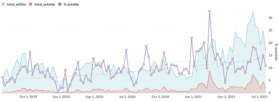
The graph above is actual data from the Hubble platform. Over two years, the amount of work done outside work hours increased from 5% to 15% (a 3x increase). Given this information, we then work with HR to protect our staff’s well-being.

Protecting against knowledge decay

“Bus Factor” is the number of engineers that have to be run over by a bus for the project to fail. The higher the bus factor, the lower the risk is for the company. It is therefore essential for tech executives to have visibility on this. At Hubble, we monitor this by the number of commits each person does throughout his tenure for each project. Names of people and projects have been modified in the example metrics below.

Notice that Project 1 is considered low risk because John, Sheryl, and Sandy are all still in the company and have so many commits in the code that the amount of shared context they have is quite high. However, Project 4 is not as good. If Dawson leaves, Pradeep and Vishal will have a hard time filling his shoes. As the VP of Engineering, I need to de-risk the project by delegating Dawson’s responsibilities to Pradeep and Vishal so that over time, Pradeep and Vishal can handle the workload should Dawson one day decide to move on.

Consider Project 5 however where both Enrique and Carl have already left the company. Here, we see that this project is in great danger. Not only is Pragati the only one left, her leaving or falling sick will just cause the project to stop. With this data, I can now expedite hiring for this project and consider moving people from other projects into Project 5.

Protecting against defects

Another issue that often plagues engineering managers is how they can reduce defect density. A study done by Smartbear and Cisco has shown 200-400 lines of code per commit yield around 70-90% of issues found. Anything more than that reduces the capacity of the code reviewer to identify issues. Hence, it is important for engineers to see how well they perform in this metric. We compute this by the total lines of code changed each week divided by the number of commits made in that week. Here’s what a sample data looks like:

As one might observe, Anthony is doing quite well whereas Bella, Dawson, and Janise need some coaching. This will help Engineering Managers raise this in their one on ones to help improve overall team productivity.

Our software engineering analytics stack

GItlab APIs: Accessing your Gitlab data

Users of Gitlab are given the option to extract relevant data that has been created as a result of the use of its application (creating a new project/repository, creating merge requests etc.). Gitlab has a publicly-available link that documents all available REST APIs that can be called via any compatible functions. All it requires is the API URL (and corresponding query parameters) and an access token that can be created within the Gitlab web application.

In our stack, we mainly use Python to execute these Gitlab API calls. The result of these calls usually come in JSON format. Depending on which fields we wish to store as a dedicated column in a data warehouse table (more on how this is achieved in subsequent sections), we then use various objects in the pandas package to convert the inbound semi-structured data into tabular format (as a DataFrame). This multi-step workflow is managed using Apache Airflow, eventually sinking the data into Hubble’s Data Lake.

Amazon S3: Storing our latest Gitlab data with ease and with low-cost

Now that we have established a script to execute the relevant API calls, we would then require a service to persistently store the inbound data. We opted for Amazon S3 as our cloud storage solution to integrate with downstream applications like Amazon Redshift and Metabase.

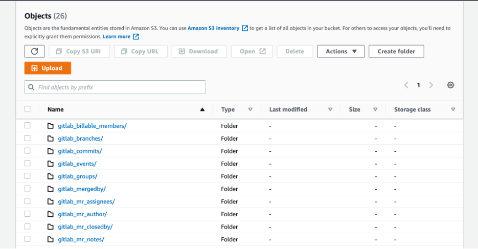
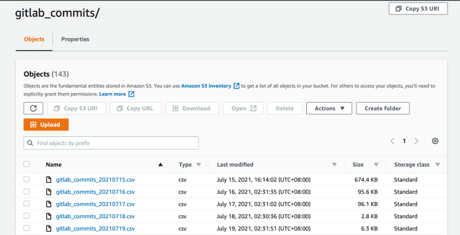
Our strategy was to turn each Gitlab API dataset response into its own dedicated table. With that, we used Python scripting to transform the original dataset structure in JSON format into a structured file format like CSV. Following this conversion, these CSV files are then stored in their own S3 sub-directories that will be read by our data warehouse application.

Amazon Redshift: Simple, secure, and fast insight on the cloud

Most data visualizations require a data source that a business intelligence tool would be able to connect to. We have selected Amazon Redshift as it fits perfectly with our existing AWS stack, integrating with our underlying data storage in Amazon S3, its distributed nature and its automated table designed to optimize query speeds.

Our Python script programmatically reads every new CSV that has been deposited in Amazon S3 into the corresponding Amazon Redshift table using the common COPY functions. Amazon Redshift’s COPY command reads the contents of an existing file and writes its contents into a Redshift table. All it requires is the fully-defined file URI, Redshift table name, and the corresponding IAM role that has the required permissions to read from the S3 bucket and write into the Redshift instance.

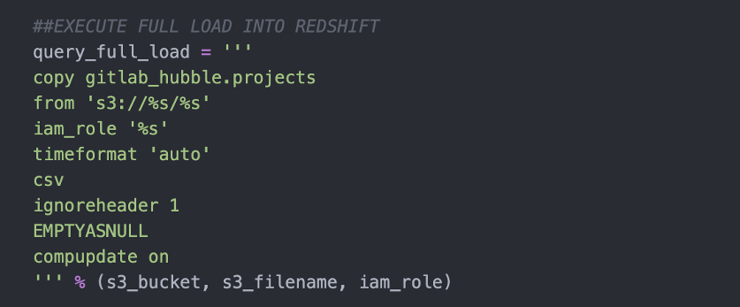
For each of the Amazon S3 sub-directories, we thus transform all the data that has been stored as S3 objects into data warehouse tables which can now be accessed and analyzed with SQL.

Apache Airflow: Orchestrating the flow of data

In order for us to establish an automatic pipeline that pulls, transforms, and stores data without manual intervention, we used Apache Airflow to orchestrate all required steps for analysis. Airflow is open-source and free to use. Using Python coding, data engineers will be able to chain multiple tasks into a collection known as a Direct Acyclic Graph (DAG). On top of that:

• Each DAG can be set to run at a given schedule (in Hubble’s use case, we run this one every day).
• Tasks can be configured to only run when one or several previous tasks have been successful (task dependencies).
• Email notifications can be set up to inform data engineers whenever a pipeline encounters an error.
• Secure storage and retrieval of any secrets or connection parameters required for calling the necessary APIs.

Metabase: Free and Open Source Data Visualization

Our final step in our analytics stack is to integrate a data visualization tool to Amazon Redshift. We used Metabase as our tool of choice because it is a free open-source application (using its basic features are free of charge). It also provides data access control by allowing the creation of different user groups and permission settings to manage which groups have access to which data warehouse schemas or tables. Metabase supports more complex analytics by allowing custom SQL queries to generate required result sets, and simple export functions into CSV and Excel file formats are also available.

Overall, we were quite happy with the results. Thanks to Amazon Redshift, we are now able to easily see the performance of our engineering team and be more data-driven in how we approach our execution. With our setup, we are now able to act on problems before they happen. For example, we are able to proactively monitor which projects are at risk, therefore allowing us to hire more engineers to sandbag potential departures. Likewise, because we’re able to nudge the engineers to keep their commit size within the ideal lines of code, we have also seen our Change Failure Rate improve by 300% from July to November. We felt that it is tremendously important to measure what matters, and AWS made this seamless for us to do.

Advice to Other Startups

One might think that a startup is always strapped with resources. Although there are stacks of things to do, it is important for the team to take a step back and evaluate what work will yield the biggest delta in terms of where we are to where we ought to be. It is likewise important for startups to have a close-knit relationship between departments; the engineering team was able to work with HR to understand key HR metrics that were otherwise difficult to analyze manually. There is nevert really a “right time” to start doing Software Engineering Analytics, but that right time may come when it is the highest item in the overall people operations priority list.