AWS News Blog
Amazon Redshift ML Is Now Generally Available – Use SQL to Create Machine Learning Models and Make Predictions from Your Data
|
|
With Amazon Redshift, you can use SQL to query and combine exabytes of structured and semi-structured data across your data warehouse, operational databases, and data lake. Now that AQUA (Advanced Query Accelerator) is generally available, you can improve the performance of your queries by up to 10 times with no additional costs and no code changes. In fact, Amazon Redshift provides up to three times better price/performance than other cloud data warehouses.
But what if you want to go a step further and process this data to train machine learning (ML) models and use these models to generate insights from data in your warehouse? For example, to implement use cases such as forecasting revenue, predicting customer churn, and detecting anomalies? In the past, you would need to export the training data from Amazon Redshift to an Amazon Simple Storage Service (Amazon S3) bucket, and then configure and start a machine learning training process (for example, using Amazon SageMaker). This process required many different skills and usually more than one person to complete. Can we make it easier?
Today, Amazon Redshift ML is generally available to help you create, train, and deploy machine learning models directly from your Amazon Redshift cluster. To create a machine learning model, you use a simple SQL query to specify the data you want to use to train your model, and the output value you want to predict. For example, to create a model that predicts the success rate for your marketing activities, you define your inputs by selecting the columns (in one or more tables) that include customer profiles and results from previous marketing campaigns, and the output column you want to predict. In this example, the output column could be one that shows whether a customer has shown interest in a campaign.
After you run the SQL command to create the model, Redshift ML securely exports the specified data from Amazon Redshift to your S3 bucket and calls Amazon SageMaker Autopilot to prepare the data (pre-processing and feature engineering), select the appropriate pre-built algorithm, and apply the algorithm for model training. You can optionally specify the algorithm to use, for example XGBoost.
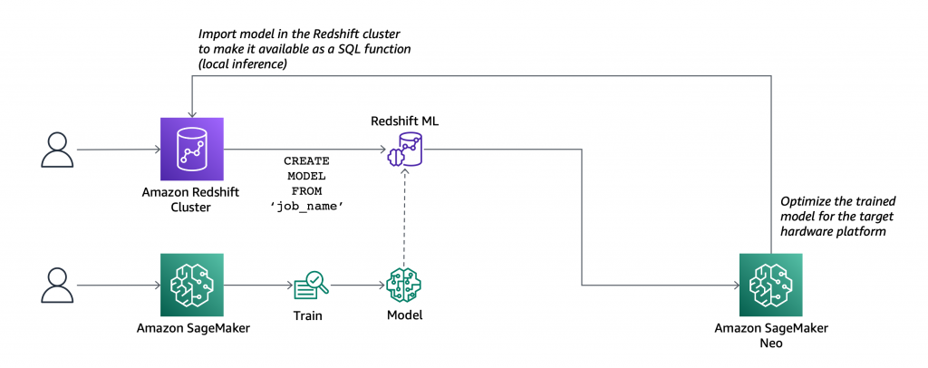
Redshift ML handles all of the interactions between Amazon Redshift, S3, and SageMaker, including all the steps involved in training and compilation. When the model has been trained, Redshift ML uses Amazon SageMaker Neo to optimize the model for deployment and makes it available as a SQL function. You can use the SQL function to apply the machine learning model to your data in queries, reports, and dashboards.
Redshift ML now includes many new features that were not available during the preview, including Amazon Virtual Private Cloud (Amazon VPC) support. For example:
- You can now import a SageMaker model into your Amazon Redshift cluster (local inference).
- You can also create SQL functions that use existing SageMaker endpoints to make predictions (remote inference). In this case, Redshift ML is batching calls to the endpoint to speed up processing.
Before looking into how to use these new capabilities in practice, let’s see the difference between Redshift ML and similar features in AWS databases and analytics services.
| ML Feature | Data | Training
from SQL |
Predictions
using SQL Functions |
| Amazon Redshift ML |
Data warehouse Federated relational databases S3 data lake (with Redshift Spectrum) |
Yes, using
Amazon SageMaker Autopilot |
Yes, a model can be imported and executed inside the Amazon Redshift cluster, or invoked using a SageMaker endpoint. |
| Amazon Aurora ML | Relational database
(compatible with MySQL or PostgreSQL) |
No |
Yes, using a SageMaker endpoint. A native integration with Amazon Comprehend for sentiment analysis is also available. |
| Amazon Athena ML |
S3 data lake Other data sources can be used through Athena Federated Query. |
No | Yes, using a SageMaker endpoint. |
Building a Machine Learning Model with Redshift ML
Let’s build a model that predicts if customers will accept or decline a marketing offer.
To manage the interactions with S3 and SageMaker, Redshift ML needs permissions to access those resources. I create an AWS Identity and Access Management (IAM) role as described in the documentation. I use RedshiftML for the role name. Note that the trust policy of the role allows both Amazon Redshift and SageMaker to assume the role to interact with other AWS services.
From the Amazon Redshift console, I create a cluster. In the cluster permissions, I associate the RedshiftML IAM role. When the cluster is available, I load the same dataset used in this super interesting blog post that my colleague Julien wrote when SageMaker Autopilot was announced.
The file I am using (bank-additional-full.csv) is in CSV format. Each line describes a direct marketing activity with a customer. The last column (y) describes the outcome of the activity (if the customer subscribed to a service that was marketed to them).
Here are the first few lines of the file. The first line contains the headers.
I store the file in one of my S3 buckets. The S3 bucket is used to unload data and store SageMaker training artifacts.
Then, using the Amazon Redshift query editor in the console, I create a table to load the data.
CREATE TABLE direct_marketing (
	age DECIMAL NOT NULL,
	job VARCHAR NOT NULL,
	marital VARCHAR NOT NULL,
	education VARCHAR NOT NULL,
	credit_default VARCHAR NOT NULL,
	housing VARCHAR NOT NULL,
	loan VARCHAR NOT NULL,
	contact VARCHAR NOT NULL,
	month VARCHAR NOT NULL,
	day_of_week VARCHAR NOT NULL,
	duration DECIMAL NOT NULL,
	campaign DECIMAL NOT NULL,
	pdays DECIMAL NOT NULL,
	previous DECIMAL NOT NULL,
	poutcome VARCHAR NOT NULL,
	emp_var_rate DECIMAL NOT NULL,
	cons_price_idx DECIMAL NOT NULL,
	cons_conf_idx DECIMAL NOT NULL,
	euribor3m DECIMAL NOT NULL,
	nr_employed DECIMAL NOT NULL,
	y BOOLEAN NOT NULL
);
I load the data into the table using the COPY command. I can use the same IAM role I created earlier (RedshiftML) because I am using the same S3 bucket to import and export the data.
Now, I create the model straight form the SQL interface using the new CREATE MODEL statement:
CREATE MODEL direct_marketing
FROM direct_marketing
TARGET y
FUNCTION predict_direct_marketing
IAM_ROLE 'arn:aws:iam::123412341234:role/RedshiftML'
SETTINGS (
  S3_BUCKET 'my-bucket'
);
In this SQL command, I specify the parameters required to create the model:
FROM– I select all the rows in thedirect_marketingtable, but I can replace the name of the table with a nested query (see example below).TARGET– This is the column that I want to predict (in this case,y).FUNCTION– The name of the SQL function to make predictions.IAM_ROLE– The IAM role assumed by Amazon Redshift and SageMaker to create, train, and deploy the model.S3_BUCKET– The S3 bucket where the training data is temporarily stored, and where model artifacts are stored if you choose to retain a copy of them.
Here I am using a simple syntax for the CREATE MODEL statement. For more advanced users, other options are available, such as:
MODEL_TYPE– To use a specific model type for training, such as XGBoost or multilayer perceptron (MLP). If I don’t specify this parameter, SageMaker Autopilot selects the appropriate model class to use.PROBLEM_TYPE– To define the type of problem to solve: regression, binary classification, or multiclass classification. If I don’t specify this parameter, the problem type is discovered during training, based on my data.OBJECTIVE– The objective metric used to measure the quality of the model. This metric is optimized during training to provide the best estimate from data. If I don’t specify a metric, the default behavior is to use mean squared error (MSE) for regression, the F1 score for binary classification, and accuracy for multiclass classification. Other available options are F1Macro (to apply F1 scoring to multiclass classification) and area under the curve (AUC). More information on objective metrics is available in the SageMaker documentation.
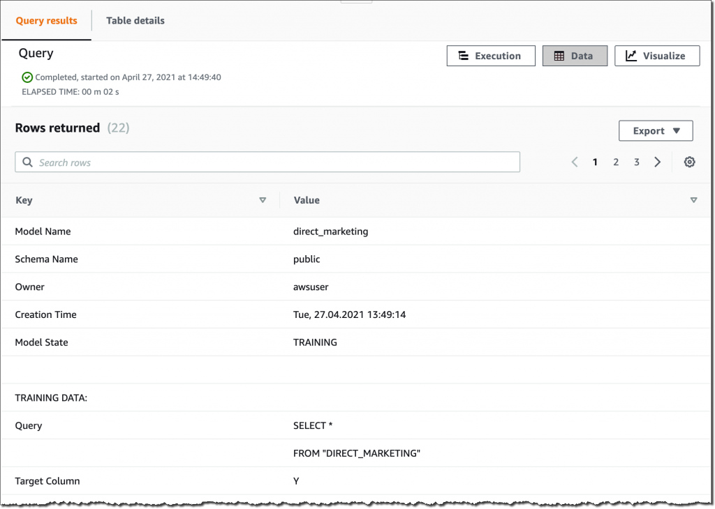
Depending on the complexity of the model and the amount of data, it can take some time for the model to be available. I use the SHOW MODEL command to see when it is available:
When I execute this command using the query editor in the console, I get the following output:
As expected, the model is currently in the TRAINING state.
When I created this model, I selected all the columns in the table as input parameters. I wonder what happens if I create a model that uses fewer input parameters? I am in the cloud and I am not slowed down by limited resources, so I create another model using a subset of the columns in the table:
CREATE MODEL simple_direct_marketing
FROM (
        SELECT age, job, marital, education, housing, contact, month, day_of_week, y
 	  FROM direct_marketing
)
TARGET y
FUNCTION predict_simple_direct_marketing
IAM_ROLE 'arn:aws:iam::123412341234:role/RedshiftML'
SETTINGS (
  S3_BUCKET 'my-bucket'
);
After some time, my first model is ready, and I get this output from SHOW MODEL. The actual output in the console is in multiple pages, I merged the results here to make it easier to follow:
From the output, I see that the model has been correctly recognized as BinaryClassification, and F1 has been selected as the objective. The F1 score is a metrics that considers both precision and recall. It returns a value between 1 (perfect precision and recall) and 0 (lowest possible score). The final score for the model (validation:f1) is 0.79. In this table I also find the name of the SQL function (predict_direct_marketing) that has been created for the model, its parameters and their types, and an estimation of the training costs.
When the second model is ready, I compare the F1 scores. The F1 score of the second model is lower (0.66) than the first one. However, with fewer parameters the SQL function is easier to apply to new data. As is often the case with machine learning, I have to find the right balance between complexity and usability.
Using Redshift ML to Make Predictions
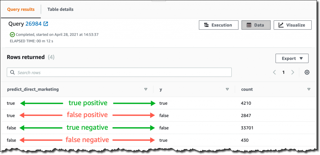
Now that the two models are ready, I can make predictions using SQL functions. Using the first model, I check how many false positives (wrong positive predictions) and false negatives (wrong negative predictions) I get when applying the model on the same data used for training:
SELECT predict_direct_marketing, y, COUNT(*)
  FROM (SELECT predict_direct_marketing(
                   age, job, marital, education, credit_default, housing,
                   loan, contact, month, day_of_week, duration, campaign,
                   pdays, previous, poutcome, emp_var_rate, cons_price_idx,
                   cons_conf_idx, euribor3m, nr_employed), y
          FROM direct_marketing)
 GROUP BY predict_direct_marketing, y;
The result of the query shows that the model is better at predicting negative rather than positive outcomes. In fact, even if the number of true negatives is much bigger than true positives, there are much more false positives than false negatives. I added some comments in green and red to the following screenshot to clarify the meaning of the results.
Using the second model, I see how many customers might be interested in a marketing campaign. Ideally, I should run this query on new customer data, not the same data I used for training.
SELECT COUNT(*)
  FROM direct_marketing
 WHERE predict_simple_direct_marketing(
           age, job, marital, education, housing,
           contact, month, day_of_week) = true;
Wow, looking at the results, there are more than 7,000 prospects!
Availability and Pricing
Redshift ML is available today in the following AWS Regions: US East (Ohio), US East (N Virginia), US West (Oregon), US West (San Francisco), Canada (Central), Europe (Frankfurt), Europe (Ireland), Europe (Paris), Europe (Stockholm), Asia Pacific (Hong Kong) Asia Pacific (Tokyo), Asia Pacific (Singapore), Asia Pacific (Sydney), and South America (São Paulo). For more information, see the AWS Regional Services list.
With Redshift ML, you pay only for what you use. When training a new model, you pay for the Amazon SageMaker Autopilot and S3 resources used by Redshift ML. When making predictions, there is no additional cost for models imported into your Amazon Redshift cluster, as in the example I used in this post.
Redshift ML also allows you to use existing Amazon SageMaker endpoints for inference. In that case, the usual SageMaker pricing for real-time inference applies. Here you can find a few tips on how to control your costs with Redshift ML.
To learn more, you can see this blog post from when Redshift ML was announced in preview and the documentation.
Start getting better insights from your data with Redshift ML.
— Danilo


