Real World AWS Scalability

This is a guest post from Linda Hedges, Principal SA, High Performance Computing.

—–
One question we often hear is, “How well will my application scale on AWS?” For high performance computing (HPC) workloads that cross multiple nodes, the cluster network is at the heart of scalability concerns.

AWS uses advanced Ethernet networking technology, which, like all things AWS, is designed for scale, security, high availability, and low cost. This network is exceptional and continues to benefit from Amazon’s rapid pace of development. Again and again, customers find that the most demanding applications run very well on AWS!

Many have speculated that highly coupled workloads require a name-brand network fabric to achieve good performance. For most applications, this is simply not the case. As with all clusters, the devil is in the details and some applications benefit from cluster tuning.

This post discusses the scalability of a representative, real-world application and provides a few performance tips for achieving excellent application performance using STAR-CCM+ as an example. For more HPC-specific information, see High Performance Computing.

Computational fluid dynamics at TLG Aerospace

TLG Aerospace, a Seattle-based aerospace engineering services company, runs most of their STAR-CCM+ computational fluid dynamics (CFD) cases on AWS. For a detailed case study describing TLG Aerospace’s experience and the results they achieved, see TLG Aerospace.

This post uses one of their CFD cases as an example to understand AWS scalability. By leveraging Amazon EC2 Spot Instances, which allow customers to purchase unused capacity at significantly reduced rates, TLG Aerospace consistently achieves an 80% cost savings compared to their previous cloud and on-premises HPC cluster options. TLG Aerospace experiences solid value, terrific scale-up, and nearly limitless case throughput—all with no queue wait!

Scale-up

HPC applications such as CFD depend heavily on the application’s ability to scale compute tasks efficiently in parallel across multiple compute resources. Parallel performance is often evaluated by determining an application’s scale-up. Scale-up is a function of the number of processors used and is defined as the time it takes to complete a run on one processor, divided by the time it takes to complete the same run on the number of processors used for the parallel run.

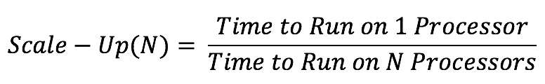
As an example, consider an application with a time to completion, or turn-around time of 32 hours when run on one processor. If the same application runs in one hour when run on 32 processors, then the scale-up is 32 hours of time on 1 processor / 1 hour time on 32 processors, or equal to 32 for 32 processes. Scaling is considered to be excellent when the scale-up is close to or equal to the number of processors on which the application is run.

If the same application took 8 hours to complete on 32 processors, it would have a scale-up of only 4: 32 (time on one processor) / 8 (time to complete on 32 processors). A scale-up of 4 on 32 processors is considered to be poor.

Strong scaling vs. weak scaling

In addition to characterizing the scale-up of an application, scalability can be further characterized as “strong” or “weak”. Note that the term “weak”, as used here, does not mean inadequate or bad but is a technical term facilitating the description of the type of scaling that is sought.

Strong scaling offers a traditional view of application scaling, where a problem size is fixed and spread over an increasing number of processors. As more processors are added to the calculation, good strong scaling means that the time to complete the calculation decreases proportionally with increasing processor count.

In comparison, weak scaling does not fix the problem size used in the evaluation, but purposely increases the problem size as the number of processors also increases. The ratio of the problem size to the number of processors on which the case is run is held constant. For a CFD calculation, problem size most often refers to the size of the grid or mesh for a similar configuration.

An application demonstrates good weak scaling when the time to complete the calculation remains constant as the ratio of compute effort to the number of processors is held constant. Weak scaling offers insight into how an application behaves with varying case size.

Scale-up as a function of increasing processor count is shown in Figure 1 for the STAR-CCM+ case data provided by TLG Aerospace. This is a demonstration of “strong” scalability. The blue line shows what ideal or perfect scalability looks like. The purple triangles show the actual scale-up for the case as a function of increasing processor count. Excellent scaling is seen to well over 400 processors for this modest-sized 16M cell case, as evidenced by the closeness of these two curves. This example was run on Amazon EC2 c3.8xlarge instances, each an Intel E5-2680, providing either 16 cores or 32 Hyper-Threading processors using Intel Hyper-Threading Technology (HTT).

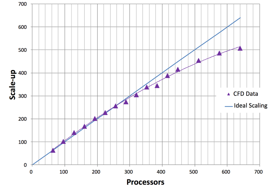
Figure 1: Strong Scaling Demonstrated for a 16M Cell STARCCM+ CFD Calculation

Threads vs. cores

AWS customers can choose to run their applications on either threads or cores. For an application like STAR-CCM+, excellent linear scaling can be seen when using either threads or cores, though we always recommend testing specific cases and applications.

For this example, threads were chosen as the processing basis. Running on threads offered a few percentage points in performance improvement when compared to running the same case on cores. Note that the number of available cores is equal to half of the number of available threads.

Processor counts

The scalability of real-world problems is directly related to the ratio of the compute effort per-core to the time required to exchange data across the network. The number of grid cells or mesh size of a CFD case provides a strong indication of how much computational effort is required for a solution. Thus, larger cases scale to even greater processor counts than for the modest sized case discussed here.

STAR-CCM+ has been shown to demonstrate exceptional “weak” scaling on AWS. That’s not shown here, though weak scaling is reflected in Figure 2 by plotting the cells per processor on the horizontal axis. The purple line in Figure 2 shows scale-up as a function of grid cells per processor. The vertical axis for scale-up is on the left-hand side of the graph as indicated by the purple arrow. The green line in Figure 2 shows efficiency as a function of grid cells per processor. The vertical axis for efficiency is shown on the right side of the graph and is indicated with a green arrow. Efficiency is defined as the scale-up divided by the number of processors used in the calculation.

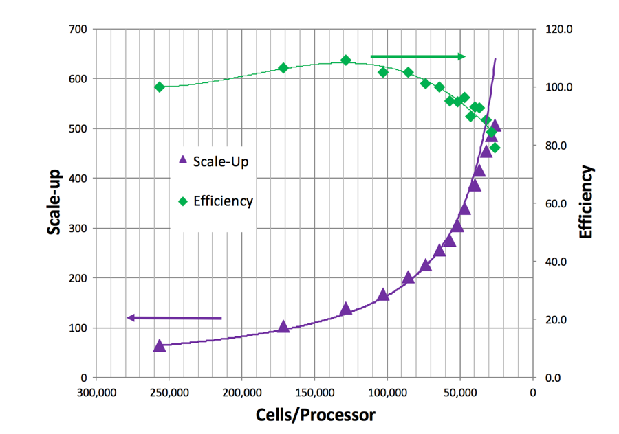
Figure 2: Scale-up and Efficiency as a Function of Cells per Processor

Weak scaling is evidenced by considering the number of grid cells per processor as a measure of compute effort. Holding the grid cells per processor constant while increasing total case size demonstrates weak scaling. Weak scaling is not shown here, because only one CFD case is used.

Efficiency

Fewer grid cells per processor means reduced computational effort per processor. Maintaining efficiency while reducing cells per processor demonstrates the excellent strong scalability of STAR-CCM+ on AWS.

Efficiency remains at about 100% between approximately 250,000 grid cells per thread (or processor) and 100,000 grid cells per thread. Efficiency starts to fall off at about 100,000 grid cells per thread. An efficiency of at least 80% is maintained until 25,000 grid cells per thread. Decreasing grid cells per processor leads to decreased efficiency because the total computational effort per processor is reduced. Note that the perceived ability to achieve more than 100% efficiency (here, at about 150,000 cells per thread) is common in scaling studies, is case-specific, and often related to smaller effects such as timing variation and memory caching.

Turn-around time and cost

Plots of scale-up and efficiency offer an understanding about how a case or application scales. The bottom line, though, is that what really matters to most HPC users is case turn-around time and cost. A plot of turn-around time versus CPU cost for this case is shown in Figure 3. As the number of threads are increased, the total turn-around time decreases. But as the number of threads increases, the inefficiency also increases, which leads to increased costs. The cost shown is based on a typical Spot price for the c3.8xlarge and only includes the computational costs. Small costs are also incurred for data storage. Note that the Spot market price varies from day to day.

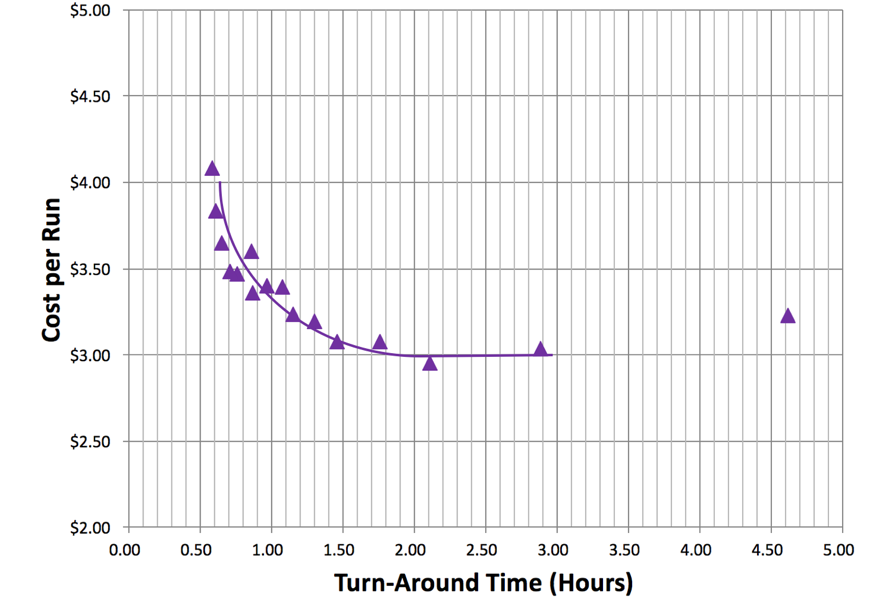
Figure 3: Cost for per Run Based on Spot Pricing ($0.35 per hour for c3.8xlarge) as a function of Turn-around Time

Minimum cost and turn-around time were achieved with approximately 100,000 cells per thread. Many users choose a cell count per thread to achieve the lowest possible cost. Others may choose a cell count per thread to achieve the fastest turn-around time.

If a run is desired in 1/3rd the time of the lowest price point, it can be achieved with approximately 25,000 cells per thread. (Note that many users run STAR-CCM+ with significantly fewer cells per thread than this.) While this increases the compute cost, other concerns—such as license costs or schedules—can be overriding factors. For this 16M cell case, the added inefficiency results in an increase in run price from $3 to $4 for computing. Many find the reduced turn-around time well worth the price of the additional instances.

Cluster tuning tips

As with any cluster, good performance requires attention to the details of the cluster setup. While AWS allows for the quick set up and take down of clusters, performance is affected by many of the specifics in that setup. This post provides some examples.

Placement groups

On AWS, a placement group is a grouping of instances within a single Availability Zone that allow for low latency between the instances. Placement groups are recommended for all applications where low latency is a requirement. A placement group was used to achieve the best performance from STAR-CCM+. For more information, see Placement Groups in the Amazon EC2 User Guide for Linux Instances.

Amazon Linux OS

Amazon Linux is a version of Linux maintained by Amazon. The distribution is designed to provide a stable, secure, and highly performant environment. Amazon Linux is optimized to run on AWS and offers excellent performance for running HPC applications. For the case presented here, the operating system used was Amazon Linux. Other Linux distributions are also performant. However, we strongly recommend that for Linux HPC applications, you use a minimum of the version 3.10 Linux kernel, to be sure of using the latest Xen libraries. For more information, see Amazon Linux AMI.

Amazon EBS storage

Amazon Elastic Block Store (Amazon EBS) is a persistent, block-level storage device often used for cluster storage on AWS. EBS provides reliable block-level storage volumes that can be attached (and removed) from an Amazon EC2 instance. A standard EBS General Purpose SSD (gp2) volume is all that is required to meet the needs of STAR-CCM+, and was used for this post. Other HPC applications may require faster I/O to prevent data writes from being a bottleneck to turn-around speed but also, many HPC applications only require the less expensive throughput optimized EBS volumes. For these applications, other storage options exist. For more information, see Storage.

Intel Hyper-Threading Technology (HTT)

As mentioned previously, STAR-CCM+, like many other CFD solvers, runs well on both threads and cores. HTT can improve the performance of some MPI applications depending on the application, case, and size of the workload allocated to each thread; it may also slow performance. The one-size-fits-all nature of the static cluster compute environments means that most HPC clusters disable HTT.

Generally, computationally intensive workloads run best on cores while those that are I/O bound run best on threads. Again, a few percentage points increase in performance was discovered for this case, by running with threads. If there is no time to evaluate the effect of HTT on case performance, then we recommend that HTT be disabled. When disabled, it is important to bind the core to designated CPU, also known as processor or CPU affinity. It almost universally improves performance over unpinned cores for computationally intensive workloads.

Time Stamp Counter

Occasionally, an application includes frequent time measurement in the code; perhaps this is done for performance tuning. Under these circumstances, performance can be improved by setting the clock source to the TSC (Time Stamp Counter). This tuning was not required for this application but is mentioned here for completeness.

Summary

When you evaluate an application, we recommend using a meaningful, real world use case. A case that is too large or small won’t reflect the performance and scalability achievable in everyday operation. The only way you’ll know positively how an application will perform on AWS is to try it!

AWS offers solid strong scaling and exceptional weak scaling. Excellent performance can be achieved on AWS for most applications. In addition to low cost and quick turn-around time, important considerations for HPC also include throughput and availability. AWS offers nearly limitless throughput, security, cost-savings, and high-availability making queues a “thing of the past”. A long queue wait makes for a long case turn-around time, regardless of the scale.

If you have questions or suggestions, please comment below.