Optimizing MPI application performance on hpc7a by effectively using both EFA devices

This post was contributed by Sai Sunku, Software Engineer, Annapurna Labs, Matt Koop, Principal Engineer and Karthik Raman, Principal Performance Engineer, HPC Engineering

The hpc7a instance type is the latest generation AMD-based HPC instance type offered by AWS. It’s available in multiple sizes and offers superior performance compared to the previous generation hpc6a instance type. See our previous post for a deep dive on the hpc7a instance itself and this other post that describes the different instance sizes.

If you’re an MPI user, you’ll want to know that Hpc7a’s network bandwidth of 300 Gbps is 3x higher than hpc6a. We’ve done this by using two network cards, where each card is exposed to the user software as a different PCIe device. Effectively using the two network cards is essential for achieving the best performance on hpc7a.

In this post we’ll show you how to configure your application and MPI to use both network cards so you can achieve the greatest performance for your codes. We’ll also discuss some benchmarks you can look at to verify that you’re actually using both network cards. Finally, we’ll dig into some application results to give you a taste of the speedup you can get in your applications.

Under the hood

Let’s start with the PCIe topology. As the post on instance sizes described, all hpc7a instance sizes use the same underlying hardware, but with different cores enabled or disabled to make it easy to get the best memory bandwidth per core for most codes. The hardware is based on the 4th generation AMD EPYC (Genoa) processor with 192 physical cores in a 2-socket configuration with 96 physical cores per socket.

In multi-domain NUMA systems, not all PCIe devices are created equal. Processes can be more efficient if they use the PCIe device closest to them and avoid communication across sockets. It’s no different for EFA devices. Using the network card closest to your MPI process allows for much better performance. The topology for EFA devices is shown in Figure 1.

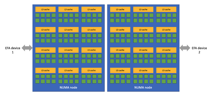
Figure 1 – Topology of the EFA devices in hpc7a. Each green square represents a processor core and the orange rectangle the L3 cache shared by 8 cores. There are two NUMA domains with 96 cores per domain connected by a high speed interconnect. The two EFA devices are associated with one NUMA node each.

Running MPI applications

The good news is that the hpc7a instance is designed to work right out of the box with your MPI for a variety of expected uses.

Many MPIs refer to using multiple network cards as “multi-rail,” where each “rail” refers to a single network card, or in our case, an EFA device. In both Open MPI and Intel MPI, when using a multi-rail configuration with EFA, each rank will be assigned a single “rail.”

This means that in a two rail setup, half of the ranks on the instance will be assigned to one rail, and the other half to the other rail. This is generally desirable, because each rank is communicating separately – and for many applications that can lead to more efficient communication. Our tests have shown that real applications can be significantly faster when they use both EFA devices and you’ll see that in the data at the end of this post, too.

If you run your application with 192 ranks on a hpc7a.96xlarge instance with one rank per core, then each rank should automatically use the correct network card. But if you choose to run your application with fewer ranks per instance (maybe your application is memory intensive or you’re optimizing for licensing costs) then you need to consider which process is running on which core. You can configure the process placement through your scheduler or MPI. But this is also exactly why we offer smaller hpc7a instance sizes with some of the cores disabled. For many applications, using a smaller instance size will assign the MPI ranks to the correct cores and thus provide the best performance.

However, if you use a bandwidth benchmark that uses only one process per instance (like the osu_bw benchmark), you can only see the bandwidth associated with a single rail. Figure 2 shows the results of osu_bw benchmark with 2 x hpc7a instances. The measured bandwidth is significantly smaller than the advertised rate of 300 Gbps. This lower bandwidth is because the benchmark is running a single rank per node. Virtually all real applications run multiple ranks per node.

How can you make sure that different ranks are assigned to different EFA devices?

If you’re using Open MPI v 4.1.0 or later or the newly released Intel MPI 2021.12, you don’t have to do much. Open MPI and the latest Intel MPI can detect the two EFA devices and use them both, exactly as you’d expect.

However, to get the same experience with Intel MPI versions 2021.11 or earlier, you need to set an environment variable I_MPI_MULTIRAL=1 and pass that environment variable to the mpirun or mpiexec command. Typically, that means running your application like this:

mpirun -genv I_MPI_MULTIRAIL=1 -n <number of processes> <your application>

Support for this environment variable was added to Intel MPI version 2021.6.

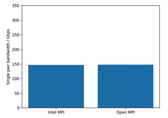
Figure 2 – OSU single pair bandwidth benchmark for Intel MPI and Open MPI. The measured bandwidth is significantly smaller than the maximum value of 300 Gbps for hpc7a.

Performance measurements

To measure the bandwidth with both EFA devices in use, we need a multi-pair bandwidth benchmark similar to the osu_mbw_mr benchmark. In this benchmark, the MPI ranks are grouped into pairs and the ranks in each pair send data to each other.

Figure 3a shows the results of an internally developed multi-pair bandwidth benchmark similar to osu_mbw_mr for two hpc7a instances with 192 ranks on each instance. With I_MPI_MULTIRAIL=0, Intel MPI was unable to take advantage of both network cards and we see a bandwidth value close to 150 Gbps. With I_MPI_MULTIRAIL=1, we see the expected value close to 300 Gbps. Open MPI shows a bandwidth close to 300 Gbps out of the box.

While bandwidth is important if your application is sending large messages, the number of messages sent, or the message rate, becomes more important for smaller messages.

Figure 3b shows the message rate for 2kiB messages. Using both EFA devices led to a significant improvement in the message rate at small message sizes as well. So whether your application sends a few large messages or many small messages, you can improve its performance by using both EFA devices.

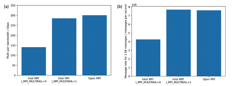
Figure 3 – Multi-pair bandwidth and message rate benchmarks for Intel MPI with I_MPI_MULTIRAIL=0, Intel MPI with I_MPI_MULTIRAIL=1 and Open MPI. The message rate is for messages 2kiB in size. Intel MPI with I_MPI_MULTIRAIL=0 is unable to take advantage of both EFA devices and shows a lower bandwidth and message rate.

Finally, let’s look at some application benchmarks to see how setting I_MPI_MULTIRAIL=1 can speed up actual applications.

Figure 4 shows the results for the CONUS 2.5km benchmark performance using WRF v4.2.2. We used the Intel compiler version 2022.1.2 and Intel MPI 2021.9.0 to compile and run WRF and calculated the speedup based on the total compute time. For 32 instances, setting I_MPI_MULTIRAIL=1 led to a 10% increase in the speedup. For 192 instances, the increase was over 30%.

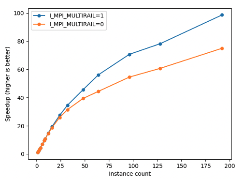
Figure 4 –Speedup in runtime for WRF CONUS 2.5km benchmark. At large instance counts, we see that I_MPI_MULTIRAIL=1 shows a higher speedup.

Finally, figure 5 shows the results for the External flow over a Formula-1 race car test-case, running on ANSYS Fluent and Intel MPI 2021.9.0. We used the solver rating to compare performance. For 48 instances, setting I_MPI_MULTIRAIL=1 boosted the solver rating by > 15%.

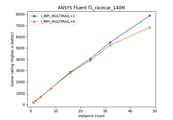
Figure 5 –Solver rating for f1_racecar_140M test case in ANSYS Fluent. At large instance counts, we see that I_MPI_MULTIRAIL=1 provides a significant boost in solver rating.

Conclusion

In this post, we talked about the PCIe topology of hpc7a instances, how MPI applications use EFA devices and how you can make tuning changes to achieve best performance on hpc7a. If you’re using Open MPI, you can get the best performance right out of the box. If you’re using Intel MPI, we suggest upgrading to the latest 2021.12 release to achieve the same outcome, or set the environment variable I_MPI_MULTIRAIL=1 in your job scripts.

We hope you get great performance from the hpc7a instances for your HPC workloads. Reach out to us at ask-hpc@amazon.com with your thoughts and questions. Happy computing!