AWS Big Data Blog
Optimizing for Star Schemas and Interleaved Sorting on Amazon Redshift
Chris Keyser is a Solutions Architect for AWS
Many organizations implement star and snowflake schema data warehouse designs and many BI tools are optimized to work with dimensions, facts, and measure groups. Customers have moved data warehouses of all types to Amazon Redshift with great success.
The Amazon Redshift team has released support for interleaved sort keys, another powerful option in its arsenal for speeding up queries. Interleaved sort keys can enhance performance on Amazon Redshift data warehouses, especially with large tables. Amazon Redshift performs well on common data models like a star or snowflake schema, third normal form (3NF), and denormalized tables.
Last year AWS published an article titled “Optimizing for Star Schemas on Amazon Redshift” that described design considerations when using star schemas.This post replaces that article and shows how interleaved sort keys may affect design decisions when implementing star schemas on Amazon Redshift. You will see many links to the Amazon Redshift Database Developer Guide, which is the authoritative technical reference and has a deeper explanation of the features and decisions highlighted in this post.
Star and snowflake schemas organize around a central fact table that contains measurements for a specific event, such as a sold item. The fact table has foreign key relationships to one or more dimension tables that contain descriptive attribute information for the sold item, such as customer or product. Snowflake schemas extend the star concept by further normalizing the dimensions into multiple tables. For example, a product dimension may have the brand in a separate table. Often, a fact table can grow quite large and will benefit from an interleaved sort key. For more information about these schema types, see star schema and snowflake schema.
Most customers experience significantly better performance when migrating their existing data models largely unchanged to Amazon Redshift due to columnar compression, flexible data distribution, and configurable sort keys. While Amazon Redshift automatically detects star schema data structures and has built-in optimizations for efficiently querying this data, you can further optimize your data model to improve query performance. The following principal areas are under your control.
- Defining how Amazon Redshift distributes data for your tables, which affects how much data moves between nodes when queried, and how load is distributed between nodes.
- Defining the type of sort key and the columns in the sort key, which determines the ordering of data stored on disk and can speed up filtering, aggregation, and joins.
- Defining the compression of data in your table, which affects the amount of disk I/O performed.
- Defining foreign key and primary key constraints, which act as hints for the query optimizer.
- Running maintenance operations to ensure optimal performance, which affects the statistics used by the query optimizer and the ordering of new data stored on disk.
- Using workload management to separate long running queries from short running queries.
- Managing the use of cursors for large result sets.
Each of these areas can affect the overall performance of your solution.
Data Distribution
Massive parallel processing (MPP) data warehouses like Amazon Redshift scale horizontally by adding compute nodes to increase compute, memory, and storage capacity. The cluster spreads data across all of the compute nodes, and the distribution style determines the method that Amazon Redshift uses to distribute the data. When a user executes SQL queries, the cluster spreads the execution across all compute nodes. The query optimizer will, where possible, optimize for operating on data local to a compute node, and minimize the amount of data that passes over the network between compute nodes.
Your choice of data distribution style and distribution key affects the amount of query computation that can occur on data local to a compute node to avoid redistributing intermediate results. When you create a table on Amazon Redshift, you specify a distribution style of EVEN, ALL, or KEY. An EVEN style spreads data across evenly all nodes in your cluster and is the default option. For a distribution style of ALL, the data for the table is put on each node, which has load performance and storage implications although it ensures that the table data will always be local on every compute node. If you specify a distribution style of KEY, then the rows with the same value for the designated DISTKEY column are placed at the same node.
Choosing a Distribution Style
Using distribution keys is a good way to optimize the performance of Amazon Redshift when you use a star schema. With an EVEN distribution, data is spread equally across all nodes in the cluster to ensure balanced processing. In many cases, simply distributing data equally using EVEN does not optimize performance as the data rows on a node for the table do not have any affinity with each other. Take an example of a fact table for ORDERS where a distribution style of EVEN is chosen. In this case, the orders for a specific customer are potentially spread across many compute nodes in the cluster. However, if the table had a distribution style of KEY and a DISTKEY of customer_id was chosen, then all of the orders for a particular customer would be stored on the same compute node. Using a distribution style of EVEN can lead to more cross-node traffic.
A good selection for a distribution key distributes data relatively evenly across nodes while collocating related data on a compute node used in joins or aggregates. When you perform a join on a column that is a distribution key for both tables, Amazon Redshift is able to run the join locally on each node with no inter-node data movement; this is because rows with the same distribution key value reside on the same node for both tables in the join. Similarly, aggregating on a distribution key performs better because the data for the aggregate column value is local to the compute node.
In a typical star schema, the fact table has foreign key relationships with multiple dimension tables, so you need to choose one of the dimensions. You would choose the foreign key for the largest frequently joined dimension as a distribution key in the fact table and the primary key in the dimension table. Make sure that the distribution keys chosen result in relatively even distribution for both tables, and if the distribution is skewed, use a different dimension. Then analyze the remaining dimensions to determine if a distribution style of ALL, KEY, or EVEN is appropriate.
For slowly changing dimensions of reasonable size, DISTSTYLE ALL is a good choice for the dimension (reasonable size in this case means up to a few million rows, and that the number of rows in the dimension table is fewer than the filtered fact table for a typical join). If you have very frequent updates to a dimension table, then DISTSTYLE ALL may not be appropriate. In this case, it is better to use a distribution style of KEY and distribute on a column that distributes data relatively evenly rather than using DISTSTYLE EVEN.
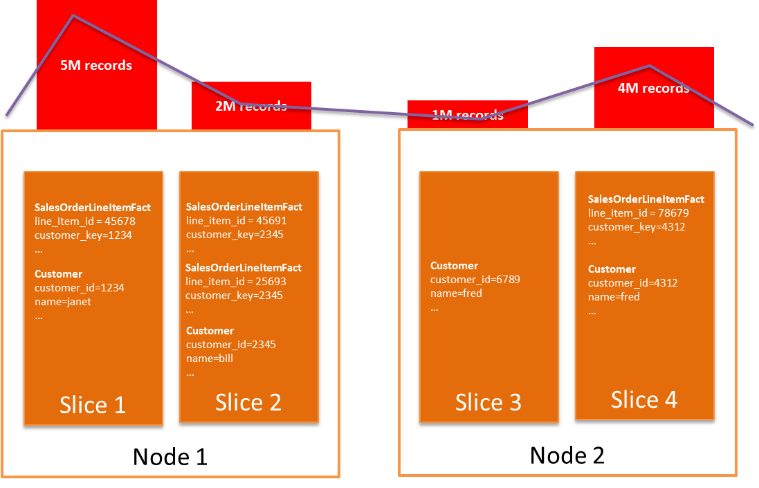
Key Distribution Style and Skew
Skew is a critical factor related to a distribution style of KEY. Skew measures the ratio between the fewest and greatest number of rows on a compute node in the cluster. A high skew indicates that you have many more rows on one (or more) of the compute nodes compared to the other nodes. Skew results in performance hotspots and negates the benefits of distributing data for node-local joins. Check your assumptions with skew; sometimes you think a column provides good distribution but in reality it does not. A common occurrence is when you don’t realize that a column is nullable, resulting in rows with null placed on one compute node. If no column provides relatively even data distribution using a KEY distribution style, then choose a style of EVEN. For examples of checking skew, see the tuning reference below.
If you need to use a style of EVEN for some of your tables, then try to form your queries to join these tables as late as possible. This results in a smaller data set, when you apply the join to the evenly distributed table, and improves performance.
For detailed guidance on choosing a distribution style, see Choosing a Data Distribution Style, especially the subsection Designating Distribution Styles, as well as the topics Choose the Best Distribution Style and the Tuning Table Design tutorial. More specific guidance on choosing distribution styles and keys can be found in the tutorial section Step 4: Select Distribution Styles.
Data Ordering with Sort Keys
A sort key determines the order of data stored on disk for your table. Amazon Redshift improves query performance when the sort key is used in the where clause (often called a filter predicate) by checking the min and max value in a block and skipping blocks of data that do not fall into the range defined by the predicate. Tables on Amazon Redshift can have only one sort key defined, with the option of multiple columns in the sort key. Amazon Redshift now offers two types of sort keys: compound and interleaved.
A compound sort key specifies precedence among the sort key columns. It sorts first by the first key, distinguishes ties using the second sort key, and so on. A compound sort key can include up to 400 columns, which are collectively used to filter data at query time. A compound sort key is useful when a prefix of the sort key columns is used to filter data in the query. If the leading key in a compound sort key is relatively unique (has high cardinality), then adding additional columns to your sort key has little impact on query performance while adding maintenance costs. A good rule of thumb is to keep the number of columns to six or fewer when using a compound sort key. There are valid situations for using more than six columns, although those situations are typically more advanced tuning options. For compound sort keys, Amazon Redshift also makes operations like group by or order by on the sort column more efficient.
Interleaved sort keys, on the other hand, treat each column with equal importance. Use interleaved sort keys when you do not know exactly which combinations of columns will be used in your queries. An interleaved sort key can contain up to 8 columns and improves query performance when any subset of the keys (in any order) are used in a filter predicate. Queries perform faster as more sort key columns are specified in the filter predicate. For example, assuming you have a sort key of 4 columns, then using 3 of the columns in your filter predicate will perform better than using 2 of the columns. In addition, tables using interleaved sort keys perform better with fewer sort keys defined. Make sure that you do not have extraneous columns when you create your sort keys.
To illustrate the uses of the sort key types, let’s say a product table uses the type, color, and size columns as the compound sort key (in that order), i.e., COMPOUND sortkey(type, color, size). If you filter on type=’shirt’ and color = ‘red’ and size = ‘xl’, then Amazon Redshift is able to take full advantage of the compound sort key. If you filter on type=’shirt’ and color = ‘red’, the compound sort key still makes the query more efficient as type and color are a leading part of the sort key (i.e., a prefix of the sort key columns). If you filter for color=’red’ and size=’xl’, then the compound sort key is limited to no impact (it may still boost performance if the leading key is low cardinality). However, if the type, color, and size columns are specified as an interleaved sort key, then the query on color and size is faster. The use of any of the interleaved sort key columns in the filter predicate improves performance, and performance gains increase for more selective queries that use multiple columns.
Choosing between an Interleaved or Compound Sort Key
There are several tradeoffs between compound and interleaved sort keys. Interleaved sort keys are slightly more costly to maintain today than compound sort keys. Compound sort keys can also improve the performance of joins, group by and order by statements, while interleaved sort keys do not. As a result, if you always query your table with a prefix of the sort keys in filter predicates, then compound sort keys will give you the best performance with lower maintenance costs. On the other hand, a good use case for an interleaved sort key is a large fact table (> 100M+ rows) where typical data query patterns use different subsets of the columns in filter predicates. Further, the benefits of the interleaved sort key increase with the table size.
Another common use case where compound sort keys are a better choice than interleaved is when you are frequently appending data in order, as in a time series table. In this case, the data in the unsorted region remains naturally sorted without the need for a vacuum operation. Interleaved sorts do not preserve this natural order, and so perform worse.
In many cases, you can take advantage of both approaches. Often, data changes frequently for recent content in your fact tables, while the bulk of historical data remains unaltered. In this situation, consider maintaining two tables: a table with an interleaved sort key for the historical fact data, and a second table containing recent data with a compound sort key, with a union view over the two tables. You will need to migrate data periodically from the recent table to the historical table.
For more information about defining sort keys, see Choosing Sort Keys and the Tuning Table Design tutorial.
Data Compression
Amazon Redshift optimizes the amount and speed of data I/O by using compression and purpose-built hardware. Amazon Redshift analyzes the first 100,000 rows of data to determine the compression settings for each column when you copy data into an empty table. Because Amazon Redshift uses a columnar design, it can choose optimal compression algorithms for each column individually based upon the data content in that column, typically yielding significantly better compression than a row-based database.
Normally, you should rely upon the Amazon Redshift logic to choose the optimal compression type, although you can also choose to override these settings. Compression helps your queries perform faster and minimizes the amount of physical storage your data consumes. If you are not using a sort key, then use automatic compression. If you are using a sort key, then not compressing the sort key may improve performance, especially if the sort key is small (for example, integer values). Calculating compression is relatively expensive. When reloading a table or moving the data to another table, consider truncating the table or using create table like syntax to avoid the automatic compression calculation.
You should periodically check compression settings if you are loading new data, because the optimal compression scheme may change as the data changes. You should use the recommendations generated by Amazon Redshift. A helpful utility for optimizing compression on your tables is the Amazon Redshift Columnar Encoding utility (https://github.com/awslabs/amazon-redshift-utils). You should periodically check compression settings if you are loading new data, because the optimal compression scheme may change as the data changes. You should use the recommendations generated by Amazon Redshift. For more information about controlling compression options, see Choosing a Column Compression Type and the Review Compression Encodings section in the Tuning Table Design tutorial.. For more information about controlling compression options, see Choosing a Column Compression Type and the Tuning Table Design tutorial.
Primary and Foreign Key Constraints
It is a best practice to declare primary and foreign key relationships between your dimension tables and fact tables for your star schema. Amazon Redshift uses this information to optimize the query by eliminating redundant joins and establishing join order. Generally, the query optimizer detects redundant joins without constraints defined if you keep statistics up to date by running the ANALYZE command as described later in this post. Often, BI applications benefit from defining constraints as well.
To avoid unexpected query results, you should ensure that the data being loaded does not violate foreign key constraints because Amazon Redshift does not enforce them. You also need to ensure that primary key uniqueness is maintained by enforcing no duplicate inserts. For example, if you load the same file twice with the copy command, Amazon Redshift will not enforce primary keys and will duplicate the rows in the table. This duplication violates the primary key constraint. For more information, see Defining Constraints.
Maintenance Operations
To maintain peak performance you must perform regular maintenance operations on a daily or weekly basis. A system view, svv_table_info, provides a lot of useful information on the performance health of your tables, including areas like table skew, percent unsorted, the quality of the current table statistics, and sort key information.
Up-to-date statistics are an essential component of efficient query performance, whether using a star schema or other data model design. To maintain peak performance, execute maintenance operations when you add or refresh data and before you tune the query performance. Use the ANALYZE command to update the statistical metadata that the query planner uses to build and choose optimal plans. Alternately, you can update statistics while loading data with the COPY command by setting the STATUPDATE option to ON. If you are loading data relatively frequently and are concerned about the maintenance overhead of a full analysis, then consider only analyzing distribution and sort keys on each COPY operation, and analyze the full table at a lower frequency, such as daily or weekly.
The VACUUM command is used to re-sort data added to non-empty tables, and to recover space freed when you delete or update a significant number of rows. Performance degrades as the unsorted region grows and data is deleted or updated. One exception is when you are using a compound sort key and table data loads are in-order append only data, in which case the table remains sorted on the disk and performance does not degrade due to sort order. The COPY operation sorts data when loading an empty table, eliminating the need to run a vacuum on initial loads. If you run both VACUUM and ANALYZE, run VACUUM first because it affects the statistics generated by ANALYZE. Vacuuming is a relatively expensive operation and should be run during periods of low load. You can allocate additional memory to vacuuming in order to speed up the process.
Monitoring for long running queries and poorly performing queries is another recommended practice. You can monitor queries using the Amazon Redshift console, and periodically check a system table, stl_alert_event_log, which flags potential performance concerns. You can see the details of a specific query execution in the console under query execution details (see Analyzing Query Execution). The visualization helps you isolate which parts of a poorly performing query are taking the most time. Another good check is for queries that are getting queued, using stl_wlm_query. Long queuing times indicate that slow running queries in your cluster are backing up other queries, either due to an unexpected poorly performing query that requires optimization, or a need to separate big queries and small queries that are expected in the cluster, using workload management.
For more information, see Vacuuming Tables, Analyzing Tables, and Performing a Deep Copy.
Workload Management
Although there is nothing specific to star schemas related to workload management, it’s worth mentioning when discussing performance considerations. Amazon Redshift provides workload management that lets you segment longer running, more resource-intensive queries from shorter running queries. You can separate longer running queries, like those associated with batch operations or report generation, from shorter running queries, like those associated with dashboards or data exploration. This helps keep applications that require responsive queries from being backed up by long-running queries. You can also allocate more memory to queues handling more intensive queries, to boost their performance. For more information about workload management, see Tutorial: Configuring Workload Management (WLM) Queues to Improve Query Processing and Implementing Workload Management.
Cursors and Drivers
Cursors are another case where there are no specific concerns related to star schemas, but they are worth a mention. When queries are issued, the driver retrieves the results into memory, and then returns the result to the application. When large results are returned, this can adversely affect the client application by consuming too much memory. When cursors are used, results are retrieved a chunk at a time and consumed by the client application, reducing the impact on memory. However, using cursors consumes resources on the leader node of the cluster, and therefore Amazon Redshift limits the total size of results for cursors (result set sizes are still very large, and vary depending upon the cluster node type used). You can determine the number of concurrent cursors used by adjusting the maximum size of a result set. By decreasing the maximum size, you increase cursor concurrency. For more information about the impact of using cursors, and configuring max_cursor_result_set_size see Fetch.
AWS recently launched free ODBC and JDBC drivers optimized for use with Amazon Redshift. These drivers improve performance over the use of open source drivers, and are more memory efficient. The drivers have an additional mode (odbc: single row mode, jdbc: blocking rows mode), which retrieves results one row or a few rows at time without requiring cursors. When loading large data sets, you can now use either cursors or one of the new modes. Both approaches limit the impact on client memory by not retrieving the full data set into memory. The use of cursors has certain restrictions with concurrency and maximum result size that depends upon the cluster type. For more information, see DECLARE. The use of single row or blocking row mode is slower than cursors for large data sets because results are pulled back a single or few rows at time, while avoiding the concurrency and size restrictions that cursors incur.
Conclusion
Star and snowflake schemas run well on Amazon Redshift, and the addition of interleaved sort keys further enhances performance by reducing I/O for a wider range of filter predicates on a table when needed. Customers have had great results running many different data models on Amazon Redshift. If you are using Amazon Redshift, then interleaved sort keys can help your queries run even faster. If you haven’t tried Amazon Redshift yet, it’s easy and you can try it for free for 60 days. Make sure to check it out.
If you have questions or suggestions, please leave a comment below.
Related:
Best Practices for Micro-Batch Loading on Amazon Redshift