Aligning Cloud Costs with the General Ledger for Accurate Financial Analysis

Mastering the art of cloud finance is critical to unlocking cloud business value. Alignment between a company’s cloud costs and general ledger (GL) is key to ensuring accurate financial reporting and budget management. Finance professionals are already familiar with variance analysis and explaining spend timing. However, the decentralized nature of cloud consumption can present challenges to monthly reconciliation, leading to difficulties in cost transparency and ownership.

Accounting and Central Finance policies can impact the posting of cloud cost entries to the GL, leading to disconnects between AWS Cost and Usage Reports (CUR) data and the GL. Therefore, it is important to understand potential variance drivers.

This blog, aimed at the cloud finance community, will focus on three potential factors driving variances between the AWS CUR and the GL:

1. Corporate closing calendar
2. Accounting policies and the amortization schedule for commitment-based purchases
3. AWS Marketplace purchases or AWS Support fees after commitment-based purchases

Additionally, we’ll share an example variance analysis showing the separation of cloud cost drivers from financial process drivers to tell the month over month story.

Whether you are actually posting the cloud cost entries, or preparing variance analysis reports for leadership, we’ll explore the practical aspects of cloud finance built on real-world examples of the monthly closing process. Our aim is to help you ensure your organization’s decision-makers focus on cloud cost trends rather than spend timing or other non-cloud consumption variances.

Variances due to corporate closing calendar

Your Accounting and Central Finance teams set the corporate closing calendar outlining various monthly tasks and expected timing. Of particular importance for cloud costs is the timing of posting monthly entries and the initial monthly variance analysis for leadership. According to the report timeline, AWS finalizes your account’s usage and charges after issuing an invoice at the end of the month. Any refunds, credits, or AWS Support fees based on final usage may not be reflected until the sixth or seventh business day of the following month.

However, your corporate closing calendar may set the expectation to have cloud cost entries posted anywhere between two business days (BD) before the close of the month (BD-2) to the fifth business day of the following month (BD+5). Earlier entries provide more time for variance analysis, but require more cost estimation using data not yet finalized. Figure 1 shows corporate closing calendar activities and where they may fall on the timeline in relationship to a finalized AWS invoice.

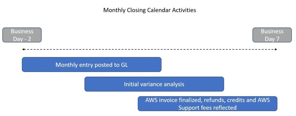
Figure 1. Example corporate closing activities and the finalized AWS invoice

Regardless of the timing, your finance team is likely having to make a partial estimate of the final cloud bill before all charges are finalized.  Therefore, the monthly entry, which we’ll call your ‘target,’ will be a combination of current month actuals plus estimated cost plus a true-up of any variance between the prior month’s estimate and prior month actuals once finalized (Figure 2).

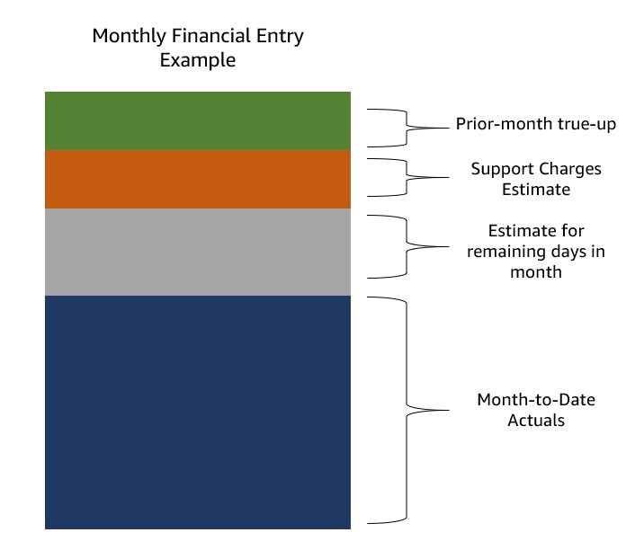
Figure 2. Common cost components of the monthly financial entry

If your corporate timing necessitates estimating costs before the CUR is finalized, the estimation method of the month-end target can lead to variances. One method is to calculate the month-to-date average daily cost and extrapolate for the total month, as a blended average.  This can be done quickly, but may lose the daily granularity for services with high weekend elasticity or incorporate one-time cost fluctuations which skew the average cost.  A more granular method is to extrapolate based on a one-week look back period, which will capture any weekend elasticity, but requires a more complex model.

To highlight the variance between estimation methods, let’s assume our financial entry must post one business day before the close of the month (BD-1) in a 31-day month, and BD-1 falls on a Friday. Figure 3 shows a $104/day weekday average, and a $91/day weekend average, resulting in a $100/day blended average ($2,808 spend / 28 days).

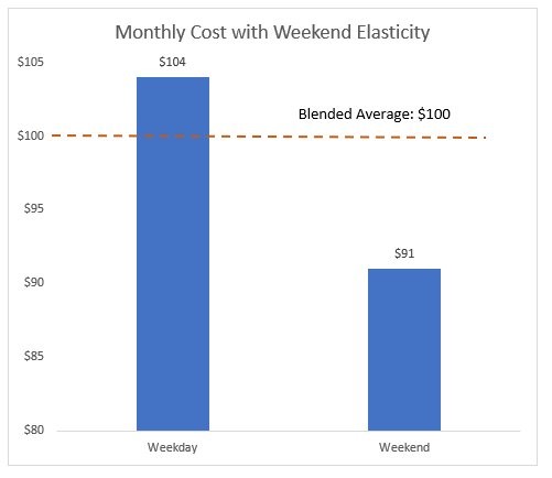
Figure 3. Daily cost average to highlight variances between extrapolation methods

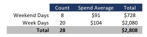
Figure 4. Daily cost average and month-to-date actuals (all figures rounded)

Our total cost through 28 days is $2,808 (Figure4) and we need to estimate one weekday and two weekend days for our monthly entry. Here we’ll estimate our monthly target using each method.

• Blended average: we use the blended average of $100/day as the spend for our remaining three days, and add this to our month-to-date (MTD) actuals. Our monthly estimate using this method is $3,108 (3 days * $100/day + $2,808 MTD actuals).
• Granular lookback: As we are estimating Friday, Saturday, and Sunday costs, we use the prior Friday/Saturday/Sunday costs as a proxy, thus capturing weekend elasticity in our estimate. Our estimate using this method is $3,094 ($101 weekday spend + $91*2 weekend days + $2,808 MTD actuals).

As our estimate includes two weekend days, the blended average will likely overstate our total month costs. Here, the granular lookback method is ~1% lower than the blended average method

Variances between the two extrapolation methods become more magnified if you make any commitment-based purchases resulting in cost savings.  AWS Savings Plans or AWS Reserved Instances reduce your bill in exchange for a one-or-three-year spend commitment., and savings from these commitment-based purchases begin on the purchase date.

If you make a commitment-based purchase late in the month, the blended average will likely overstate your cost estimate.  Your daily costs prior to the Savings Plan or Reserved Instance purchase will be higher than the daily cost after purchase. Continuing our example from above, Figure 5 shows the impact of a Savings Plan purchase resulting in 10% savings. We would want to capture the savings impact on any extrapolation estimates we make.

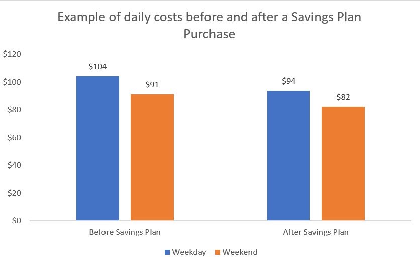
Figure 5. Daily cost average before and after a Savings Plan purchase resulting in 10% lower costs

Using a blended average, or a one-week lookback period, are just two methods of estimating cloud costs for your monthly posting. Some companies may choose to use AWS Cost Explorer forecasting or their own advanced machine-learning models for estimates, while others book their finalized cloud costs on a one-month lag. Additionally, estimate methods can change as you grow in the cloud. Perhaps simplicity works best for your current processes, as you capture any variances to your finalized actuals in the next month’s true-up entry, while you may use more advanced methods in a future state.

Variances due to accounting amortization schedule for commitment-based purchases

AWS Cost Explorer helps you understand your CUR data by showing costs either ‘unblended’ or ‘amortized,’ among other options. By default, AWS Cost Explorer shows the fees for Savings Plans or Reserved Instances on the day that you’re charged (known as ‘unblended’). Amortized costs reflect the effective cost of the upfront and monthly reservation fees spread across the billing period.

However, your accounting policy may dictate a different amortization schedule than one shown in AWS Cost Explorer. Some companies may choose to amortize purchases on an even monthly schedule, while others may operate on a 4-4-5 calendar, resulting in two 4-week months and one 5-week month per 13-week quarter.

Figure 6 shows the variances between the three types of amortization schedules on a $20/hour Savings Plan purchased as 1-year all-upfront option, for a total cost of $175,200. For each option, we assume a full month of amortization. In February, monthly amortization is 9% higher than daily or 4-4-5, assuming four weeks in February.  In March, monthly amortization is 2% lower, and 4-4-5 is 13% higher assuming five weeks, than the daily view.

Figure 6. Chart showing the Savings Plan amortized cost using three different amortization methods

The amortization start date can also drive variances. The AWS CUR shows amortized costs from the date of the purchase. However, we’ve seen accounting policies mandating the amortization of the full monthly sum, regardless of the purchase date. For purchases made near the end of the month, the variance between the AWS CUR and the GL can be significant, leading to a discrepancy between the Savings Plan cost and benefit at the beginning and ending of the purchase term. Using our $20/hour Savings Plan purchase from above, Figure 7 shows daily amortization of the purchase made with five days left in a month ($20/hour * 24 hours * 5 days) compared to amortizing the entire monthly amount ($175,200/12 months), regardless of start date.

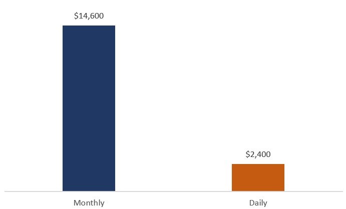
Figure 7. Chart showing an AWS Savings Plan amortized for the full month vs. from the purchase date

Variances due to AWS Marketplace purchases or AWS Support fees after commitment-based purchases

AWS Marketplace is the place to find, test, buy, and deploy software, services, and data from Independent Software Vendors (ISVs), AWS Partners, and data providers. Marketplace sellers have a number of pricing models, including annual pricing invoiced for the full amount at purchase, and contract pricing offering upfront pricing for a set term. In such cases, purchases will show in the AWS CUR as the full invoiced amount. However, companies may choose to amortize the purchase over the contract term, thereby driving a disconnect between the AWS CUR and the GL. Documentation becomes key to ensure stakeholder alignment and prevent understating or overstating costs.

For companies using one of four types of support plans, AWS Support Fees are billed monthly, with no long-term contracts, based on the monthly AWS charges. Commitment-based purchases, such as Savings Plans and Reserved Instances, are included in the monthly charges. In the case of a partial or full upfront purchase, the upfront amount is included when calculating the AWS Support fee for that month. Said another way, as you are pre-paying for usage, you’re also pre-paying for support. However, some companies may choose to amortize the AWS Support fee associated with the commitment-based purchase over the term of the commitment.

Continuing with our 1-year upfront, $20/hour Savings Plan purchase totaling $175,200, if we assume an AWS Support fee charge of 3% for the Developer plan, the Savings Plan purchase would drive an incremental $5,256 of AWS Support fees in the billing period. A company may choose to amortize that amount to match the amortization schedule of the associated Savings Plan purchase, while the AWS CUR will continue to show the incremental AWS Support fee in the billing period.

Why this matters

Challenges may arise if accounting policies or the corporate closing calendar drive material variances to the AWS CUR as different stakeholders work through variance analysis exercises. Financial process drivers may mask cloud cost impacts due to timing, and central cloud teams may struggle to explain variances outside of the AWS CUR. Therefore, understanding known potential variances between the GL and the AWS CUR can help build trust in the data among all stakeholders.

Monthly financial variance analysis will likely require tying out to the GL, but will begin with AWS CUR data. Figure 8 shows an example application-level variance analysis, with an ‘other’ category driven by the timing aspect of the monthly entry.  Using AWS Cost Explorer, Cost Intelligence Dashboards, or third-party tooling, Finance can work with the Business and Tech to understand month over month variance at the application level, ignoring any financial process impacts. The ‘other’ category is then used to tie back to the GL entry, accounting for timing and other non-cloud impacts. By separating the non-cloud variances, leadership can focus on the true variance drivers.

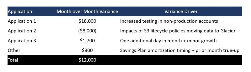
Figure 8. Monthly variance analysis example

Separating non-cloud GL impacts will also help in your forecasting process. Variances due to Savings Plan or Reserved Instances amortization, or AWS Marketplace purchases, could be material if not accounted for in your consolidation. Using our incremental AWS Support fee of $5,256 from earlier, if Accounting amortizes that amount, but the amortization is not included in the forecast, your monthly forecast will be understated even if your cloud consumption forecast aligns perfectly.

Final Thoughts

Given cloud invoice timing and the corporate closing calendar, variances between the AWS CUR and the GL are common for many companies. Our recommendation is to document your financial closing process, and educate leadership on any identified variance drivers. Calculating the variance percentage between the finalized AWS CUR and your GL entry to use as a talking point can also enhance understanding of the financial process. A data-backed statement that the GL is ‘within x% of the AWS CUR’ can help solidify trust in the process as you walk through variance drivers.

Cloud finance is challenging enough even without introducing process variances. By facilitating variance conversations focusing on cloud cost drivers, you can help drive ownership among all parties while increasing overall business value achievement.