Analyzing AWS Cost and Usage Reports with Looker and Amazon Athena

This is a guest post by Dillon Morrison at Looker. Looker is, in their own words, “a new kind of analytics platform–letting everyone in your business make better decisions by getting reliable answers from a tool they can use.”

As the breadth of AWS products and services continues to grow, customers are able to more easily move their technology stack and core infrastructure to AWS. One of the attractive benefits of AWS is the cost savings. Rather than paying upfront capital expenses for large on-premises systems, customers can instead pay variables expenses for on-demand services. To further reduce expenses AWS users can reserve resources for specific periods of time, and automatically scale resources as needed.

The AWS Cost Explorer is great for aggregated reporting. However, conducting analysis on the raw data using the flexibility and power of SQL allows for much richer detail and insight, and can be the better choice for the long term. Thankfully, with the introduction of Amazon Athena, monitoring and managing these costs is now easier than ever.

In the post, I walk through setting up the data pipeline for cost and usage reports, Amazon S3, and Athena, and discuss some of the most common levers for cost savings. I surface tables through Looker, which comes with a host of pre-built data models and dashboards to make analysis of your cost and usage data simple and intuitive.

Analysis with Athena

With Athena, there’s no need to create hundreds of Excel reports, move data around, or deploy clusters to house and process data. Athena uses Apache Hive’s DDL to create tables, and the Presto querying engine to process queries. Analysis can be performed directly on raw data in S3. Conveniently, AWS exports raw cost and usage data directly into a user-specified S3 bucket, making it simple to start querying with Athena quickly. This makes continuous monitoring of costs virtually seamless, since there is no infrastructure to manage. Instead, users can leverage the power of the Athena SQL engine to easily perform ad-hoc analysis and data discovery without needing to set up a data warehouse.

After the data pipeline is established, cost and usage data (the recommended billing data, per AWS documentation) provides a plethora of comprehensive information around usage of AWS services and the associated costs. Whether you need the report segmented by product type, user identity, or region, this report can be cut-and-sliced any number of ways to properly allocate costs for any of your business needs. You can then drill into any specific line item to see even further detail, such as the selected operating system, tenancy, purchase option (on-demand, spot, or reserved), and so on.

Walkthrough

By default, the Cost and Usage report exports CSV files, which you can compress using gzip (recommended for performance). There are some additional configuration options for tuning performance further, which are discussed below.

Prerequisites

If you want to follow along, you need the following resources:

AWS account
New or existing S3 bucket
Appropriate permissions for Athena to the S3 bucket

Enable the cost and usage reports

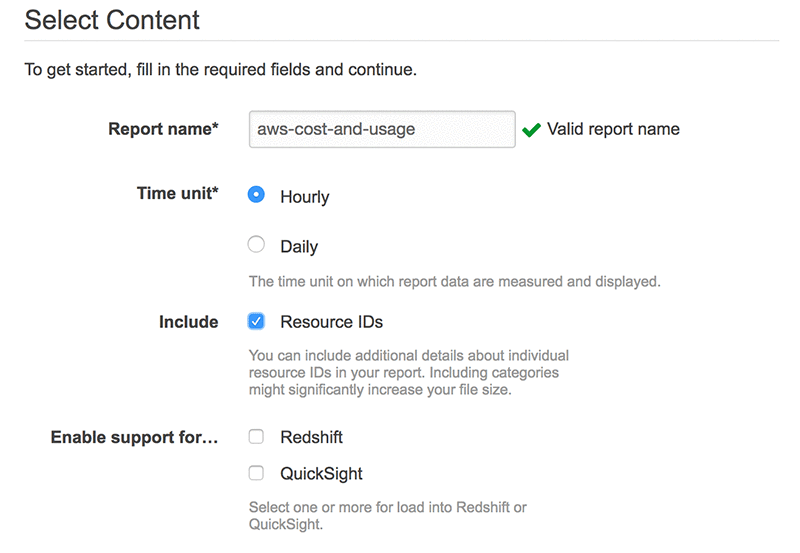
First, enable the Cost and Usage report. For Time unit, select Hourly. For Include, select Resource IDs. All options are prompted in the report-creation window.

The Cost and Usage report dumps CSV files into the specified S3 bucket. Please note that it can take up to 24 hours for the first file to be delivered after enabling the report.

Configure the S3 bucket and files for Athena querying

In addition to the CSV file, AWS also creates a JSON manifest file for each cost and usage report. Athena requires that all of the files in the S3 bucket are in the same format, so we need to get rid of all these manifest files. If you’re looking to get started with Athena quickly, you can simply go into your S3 bucket and delete the manifest file manually, skip the automation described below, and move on to the next section.

To automate the process of removing the manifest file each time a new report is dumped into S3, which I recommend as you scale, there are a few additional steps. The folks at Concurrency labs wrote a great overview and set of scripts for this, which you can find in their GitHub repo.

These scripts take the data from an input bucket, remove anything unnecessary, and dump it into a new output bucket. We can utilize AWS Lambda to trigger this process whenever new data is dropped into S3, or on a nightly basis, or whatever makes most sense for your use-case, depending on how often you’re querying the data. Please note that enabling the “hourly” report means that data is reported at the hour-level of granularity, not that a new file is generated every hour.

Following these scripts, you’ll notice that we’re adding a date partition field, which isn’t necessary but improves query performance. In addition, converting data from CSV to a columnar format like ORC or Parquet also improves performance. We can automate this process using Lambda whenever new data is dropped in our S3 bucket. Amazon Web Services discusses columnar conversion at length, and provides walkthrough examples, in their documentation.

As a long-term solution, best practice is to use compression, partitioning, and conversion. However, for purposes of this walkthrough, we’re not going to worry about them so we can get up-and-running quicker.

Set up the Athena query engine

In your AWS console, navigate to the Athena service, and click “Get Started”. Follow the tutorial and set up a new database (we’ve called ours “AWS Optimizer” in this example). Don’t worry about configuring your initial table, per the tutorial instructions. We’ll be creating a new table for cost and usage analysis. Once you walked through the tutorial steps, you’ll be able to access the Athena interface, and can begin running Hive DDL statements to create new tables.

One thing that’s important to note, is that the Cost and Usage CSVs also contain the column headers in their first row, meaning that the column headers would be included in the dataset and any queries. For testing and quick set-up, you can remove this line manually from your first few CSV files. Long-term, you’ll want to use a script to programmatically remove this row each time a new file is dropped in S3 (every few hours typically). We’ve drafted up a sample script for ease of reference, which we run on Lambda. We utilize Lambda’s native ability to invoke the script whenever a new object is dropped in S3.

For cost and usage, we recommend using the DDL statement below. Since our data is in CSV format, we don’t need to use a SerDe, we can simply specify the “separatorChar, quoteChar, and escapeChar”, and the structure of the files (“TEXTFILE”). Note that AWS does have an OpenCSV SerDe as well, if you prefer to use that.

CREATE EXTERNAL TABLE IF NOT EXISTS cost_and_usage	 (
identity_LineItemId String,
identity_TimeInterval String,
bill_InvoiceId String,
bill_BillingEntity String,
bill_BillType String,
bill_PayerAccountId String,
bill_BillingPeriodStartDate String,
bill_BillingPeriodEndDate String,
lineItem_UsageAccountId String,
lineItem_LineItemType String,
lineItem_UsageStartDate String,
lineItem_UsageEndDate String,
lineItem_ProductCode String,
lineItem_UsageType String,
lineItem_Operation String,
lineItem_AvailabilityZone String,
lineItem_ResourceId String,
lineItem_UsageAmount String,
lineItem_NormalizationFactor String,
lineItem_NormalizedUsageAmount String,
lineItem_CurrencyCode String,
lineItem_UnblendedRate String,
lineItem_UnblendedCost String,
lineItem_BlendedRate String,
lineItem_BlendedCost String,
lineItem_LineItemDescription String,
lineItem_TaxType String,
product_ProductName String,
product_accountAssistance String,
product_architecturalReview String,
product_architectureSupport String,
product_availability String,
product_bestPractices String,
product_cacheEngine String,
product_caseSeverityresponseTimes String,
product_clockSpeed String,
product_currentGeneration String,
product_customerServiceAndCommunities String,
product_databaseEdition String,
product_databaseEngine String,
product_dedicatedEbsThroughput String,
product_deploymentOption String,
product_description String,
product_durability String,
product_ebsOptimized String,
product_ecu String,
product_endpointType String,
product_engineCode String,
product_enhancedNetworkingSupported String,
product_executionFrequency String,
product_executionLocation String,
product_feeCode String,
product_feeDescription String,
product_freeQueryTypes String,
product_freeTrial String,
product_frequencyMode String,
product_fromLocation String,
product_fromLocationType String,
product_group String,
product_groupDescription String,
product_includedServices String,
product_instanceFamily String,
product_instanceType String,
product_io String,
product_launchSupport String,
product_licenseModel String,
product_location String,
product_locationType String,
product_maxIopsBurstPerformance String,
product_maxIopsvolume String,
product_maxThroughputvolume String,
product_maxVolumeSize String,
product_maximumStorageVolume String,
product_memory String,
product_messageDeliveryFrequency String,
product_messageDeliveryOrder String,
product_minVolumeSize String,
product_minimumStorageVolume String,
product_networkPerformance String,
product_operatingSystem String,
product_operation String,
product_operationsSupport String,
product_physicalProcessor String,
product_preInstalledSw String,
product_proactiveGuidance String,
product_processorArchitecture String,
product_processorFeatures String,
product_productFamily String,
product_programmaticCaseManagement String,
product_provisioned String,
product_queueType String,
product_requestDescription String,
product_requestType String,
product_routingTarget String,
product_routingType String,
product_servicecode String,
product_sku String,
product_softwareType String,
product_storage String,
product_storageClass String,
product_storageMedia String,
product_technicalSupport String,
product_tenancy String,
product_thirdpartySoftwareSupport String,
product_toLocation String,
product_toLocationType String,
product_training String,
product_transferType String,
product_usageFamily String,
product_usagetype String,
product_vcpu String,
product_version String,
product_volumeType String,
product_whoCanOpenCases String,
pricing_LeaseContractLength String,
pricing_OfferingClass String,
pricing_PurchaseOption String,
pricing_publicOnDemandCost String,
pricing_publicOnDemandRate String,
pricing_term String,
pricing_unit String,
reservation_AvailabilityZone String,
reservation_NormalizedUnitsPerReservation String,
reservation_NumberOfReservations String,
reservation_ReservationARN String,
reservation_TotalReservedNormalizedUnits String,
reservation_TotalReservedUnits String,
reservation_UnitsPerReservation String,
resourceTags_userName String,
resourceTags_usercostcategory String  


)
    ROW FORMAT DELIMITED
      FIELDS TERMINATED BY ','
      ESCAPED BY '\\'
      LINES TERMINATED BY '\n'

STORED AS TEXTFILE
    LOCATION 's3://<<your bucket name>>';

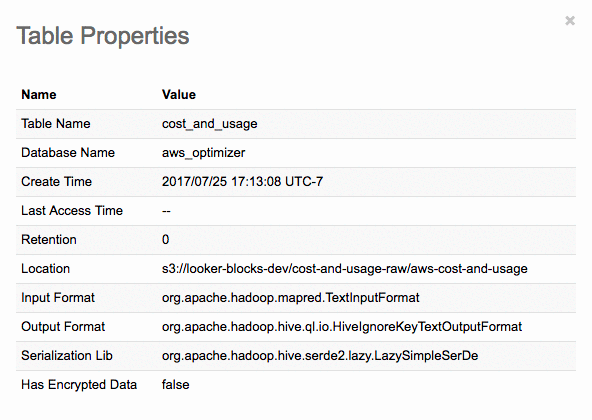
Once you’ve successfully executed the command, you should see a new table named “cost_and_usage” with the below properties. Now we’re ready to start executing queries and running analysis!

Start with Looker and connect to Athena

Setting up Looker is a quick process, and you can try it out for free here (or download from Amazon Marketplace). It takes just a few seconds to connect Looker to your Athena database, and Looker comes with a host of pre-built data models and dashboards to make analysis of your cost and usage data simple and intuitive. After you’re connected, you can use the Looker UI to run whatever analysis you’d like. Looker translates this UI to optimized SQL, so any user can execute and visualize queries for true self-service analytics.

Major cost saving levers

Now that the data pipeline is configured, you can dive into the most popular use cases for cost savings. In this post, I focus on:

Purchasing Reserved Instances vs. On-Demand Instances
Data transfer costs
Allocating costs over users or other Attributes (denoted with resource tags)

On-Demand, Spot, and Reserved Instances

Purchasing Reserved Instances vs On-Demand Instances is arguably going to be the biggest cost lever for heavy AWS users (Reserved Instances run up to 75% cheaper!). AWS offers three options for purchasing instances:

On-Demand—Pay as you use.
Spot (variable cost)—Bid on spare Amazon EC2 computing capacity.
Reserved Instances—Pay for an instance for a specific, allotted period of time.

When purchasing a Reserved Instance, you can also choose to pay all-upfront, partial-upfront, or monthly. The more you pay upfront, the greater the discount.

If your company has been using AWS for some time now, you should have a good sense of your overall instance usage on a per-month or per-day basis. Rather than paying for these instances On-Demand, you should try to forecast the number of instances you’ll need, and reserve them with upfront payments.

The total amount of usage with Reserved Instances versus overall usage with all instances is called your coverage ratio. It’s important not to confuse your coverage ratio with your Reserved Instance utilization. Utilization represents the amount of reserved hours that were actually used. Don’t worry about exceeding capacity, you can still set up Auto Scaling preferences so that more instances get added whenever your coverage or utilization crosses a certain threshold (we often see a target of 80% for both coverage and utilization among savvy customers).

Calculating the reserved costs and coverage can be a bit tricky with the level of granularity provided by the cost and usage report. The following query shows your total cost over the last 6 months, broken out by Reserved Instance vs other instance usage. You can substitute the cost field for usage if you’d prefer. Please note that you should only have data for the time period after the cost and usage report has been enabled (though you can opt for up to 3 months of historical data by contacting your AWS Account Executive). If you’re just getting started, this query will only show a few days.

SELECT 
	DATE_FORMAT(from_iso8601_timestamp(cost_and_usage.lineitem_usagestartdate),'%Y-%m') AS "cost_and_usage.usage_start_month",
	COALESCE(SUM(cost_and_usage.lineitem_unblendedcost ), 0) AS "cost_and_usage.total_unblended_cost",
	COALESCE(SUM(CASE WHEN (CASE
         WHEN cost_and_usage.lineitem_lineitemtype = 'DiscountedUsage' THEN 'RI Line Item'
         WHEN cost_and_usage.lineitem_lineitemtype = 'RIFee' THEN 'RI Line Item'
         WHEN cost_and_usage.lineitem_lineitemtype = 'Fee' THEN 'RI Line Item'
         ELSE 'Non RI Line Item'
        END = 'RI Line Item') THEN cost_and_usage.lineitem_unblendedcost  ELSE NULL END), 0) AS "cost_and_usage.total_reserved_unblended_cost",
	1.0 * (COALESCE(SUM(CASE WHEN (CASE
         WHEN cost_and_usage.lineitem_lineitemtype = 'DiscountedUsage' THEN 'RI Line Item'
         WHEN cost_and_usage.lineitem_lineitemtype = 'RIFee' THEN 'RI Line Item'
         WHEN cost_and_usage.lineitem_lineitemtype = 'Fee' THEN 'RI Line Item'
         ELSE 'Non RI Line Item'
        END = 'RI Line Item') THEN cost_and_usage.lineitem_unblendedcost  ELSE NULL END), 0)) / NULLIF((COALESCE(SUM(cost_and_usage.lineitem_unblendedcost ), 0)),0)  AS "cost_and_usage.percent_spend_on_ris",
	COALESCE(SUM(CASE WHEN (CASE
         WHEN cost_and_usage.lineitem_lineitemtype = 'DiscountedUsage' THEN 'RI Line Item'
         WHEN cost_and_usage.lineitem_lineitemtype = 'RIFee' THEN 'RI Line Item'
         WHEN cost_and_usage.lineitem_lineitemtype = 'Fee' THEN 'RI Line Item'
         ELSE 'Non RI Line Item'
        END = 'Non RI Line Item') THEN cost_and_usage.lineitem_unblendedcost  ELSE NULL END), 0) AS "cost_and_usage.total_non_reserved_unblended_cost",
	1.0 * (COALESCE(SUM(CASE WHEN (CASE
         WHEN cost_and_usage.lineitem_lineitemtype = 'DiscountedUsage' THEN 'RI Line Item'
         WHEN cost_and_usage.lineitem_lineitemtype = 'RIFee' THEN 'RI Line Item'
         WHEN cost_and_usage.lineitem_lineitemtype = 'Fee' THEN 'RI Line Item'
         ELSE 'Non RI Line Item'
        END = 'Non RI Line Item') THEN cost_and_usage.lineitem_unblendedcost  ELSE NULL END), 0)) / NULLIF((COALESCE(SUM(cost_and_usage.lineitem_unblendedcost ), 0)),0)  AS "cost_and_usage.percent_spend_on_non_ris"
FROM aws_optimizer.cost_and_usage  AS cost_and_usage

WHERE 
	(((from_iso8601_timestamp(cost_and_usage.lineitem_usagestartdate)) >= ((DATE_ADD('month', -5, DATE_TRUNC('MONTH', CAST(NOW() AS DATE))))) AND (from_iso8601_timestamp(cost_and_usage.lineitem_usagestartdate)) < ((DATE_ADD('month', 6, DATE_ADD('month', -5, DATE_TRUNC('MONTH', CAST(NOW() AS DATE))))))))
GROUP BY 1
ORDER BY 2 DESC
LIMIT 500

The resulting table should look something like the image below (I’m surfacing tables through Looker, though the same table would result from querying via command line or any other interface).

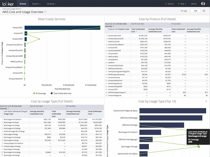
With a BI tool, you can create dashboards for easy reference and monitoring. New data is dumped into S3 every few hours, so your dashboards can update several times per day.

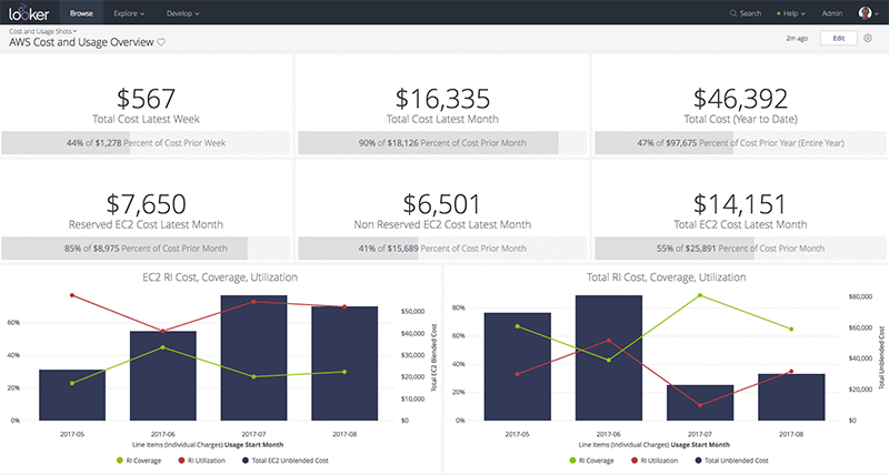
It’s an iterative process to understand the appropriate number of Reserved Instances needed to meet your business needs. After you’ve properly integrated Reserved Instances into your purchasing patterns, the savings can be significant. If your coverage is consistently below 70%, you should seriously consider adjusting your purchase types and opting for more Reserved instances.

Data transfer costs

One of the great things about AWS data storage is that it’s incredibly cheap. Most charges often come from moving and processing that data. There are several different prices for transferring data, broken out largely by transfers between regions and availability zones. Transfers between regions are the most costly, followed by transfers between Availability Zones. Transfers within the same region and same availability zone are free unless using elastic or public IP addresses, in which case there is a cost. You can find more detailed information in the AWS Pricing Docs. With this in mind, there are several simple strategies for helping reduce costs.

First, since costs increase when transferring data between regions, it’s wise to ensure that as many services as possible reside within the same region. The more you can localize services to one specific region, the lower your costs will be.

Second, you should maximize the data you’re routing directly within AWS services and IP addresses. Transfers out to the open internet are the most costly and least performant mechanisms of data transfers, so it’s best to keep transfers within AWS services.

Lastly, data transfers between private IP addresses are cheaper than between elastic or public IP addresses, so utilizing private IP addresses as much as possible is the most cost-effective strategy.

The following query provides a table depicting the total costs for each AWS product, broken out transfer cost type. Substitute the “lineitem_productcode” field in the query to segment the costs by any other attribute. If you notice any unusually high spikes in cost, you’ll need to dig deeper to understand what’s driving that spike: location, volume, and so on. Drill down into specific costs by including “product_usagetype” and “product_transfertype” in your query to identify the types of transfer costs that are driving up your bill.

SELECT 
	cost_and_usage.lineitem_productcode  AS "cost_and_usage.product_code",
	COALESCE(SUM(cost_and_usage.lineitem_unblendedcost), 0) AS "cost_and_usage.total_unblended_cost",
	COALESCE(SUM(CASE WHEN REGEXP_LIKE(cost_and_usage.product_usagetype, 'DataTransfer')    THEN cost_and_usage.lineitem_unblendedcost  ELSE NULL END), 0) AS "cost_and_usage.total_data_transfer_cost",
	COALESCE(SUM(CASE WHEN REGEXP_LIKE(cost_and_usage.product_usagetype, 'DataTransfer-In')    THEN cost_and_usage.lineitem_unblendedcost  ELSE NULL END), 0) AS "cost_and_usage.total_inbound_data_transfer_cost",
	COALESCE(SUM(CASE WHEN REGEXP_LIKE(cost_and_usage.product_usagetype, 'DataTransfer-Out')    THEN cost_and_usage.lineitem_unblendedcost  ELSE NULL END), 0) AS "cost_and_usage.total_outbound_data_transfer_cost"
FROM aws_optimizer.cost_and_usage  AS cost_and_usage

WHERE 
	(((from_iso8601_timestamp(cost_and_usage.lineitem_usagestartdate)) >= ((DATE_ADD('month', -5, DATE_TRUNC('MONTH', CAST(NOW() AS DATE))))) AND (from_iso8601_timestamp(cost_and_usage.lineitem_usagestartdate)) < ((DATE_ADD('month', 6, DATE_ADD('month', -5, DATE_TRUNC('MONTH', CAST(NOW() AS DATE))))))))
GROUP BY 1
ORDER BY 2 DESC
LIMIT 500

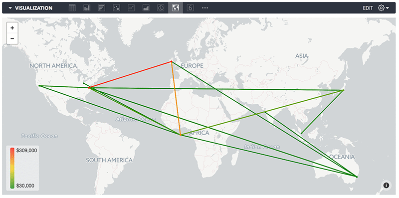
When moving between regions or over the open web, many data transfer costs also include the origin and destination location of the data movement. Using a BI tool with mapping capabilities, you can get a nice visual of data flows. The point at the center of the map is used to represent external data flows over the open internet.

Analysis by tags

AWS provides the option to apply custom tags to individual resources, so you can allocate costs over whatever customized segment makes the most sense for your business. For a SaaS company that hosts software for customers on AWS, maybe you’d want to tag the size of each customer. The following query uses custom tags to display the reserved, data transfer, and total cost for each AWS service, broken out by tag categories, over the last 6 months. You’ll want to substitute the cost_and_usage.resourcetags_customersegment and cost_and_usage.customer_segment with the name of your customer field.

SELECT * FROM (
SELECT *, DENSE_RANK() OVER (ORDER BY z___min_rank) as z___pivot_row_rank, RANK() OVER (PARTITION BY z__pivot_col_rank ORDER BY z___min_rank) as z__pivot_col_ordering FROM (
SELECT *, MIN(z___rank) OVER (PARTITION BY "cost_and_usage.product_code") as z___min_rank FROM (
SELECT *, RANK() OVER (ORDER BY CASE WHEN z__pivot_col_rank=1 THEN (CASE WHEN "cost_and_usage.total_unblended_cost" IS NOT NULL THEN 0 ELSE 1 END) ELSE 2 END, CASE WHEN z__pivot_col_rank=1 THEN "cost_and_usage.total_unblended_cost" ELSE NULL END DESC, "cost_and_usage.total_unblended_cost" DESC, z__pivot_col_rank, "cost_and_usage.product_code") AS z___rank FROM (
SELECT *, DENSE_RANK() OVER (ORDER BY CASE WHEN "cost_and_usage.customer_segment" IS NULL THEN 1 ELSE 0 END, "cost_and_usage.customer_segment") AS z__pivot_col_rank FROM (
SELECT 
	cost_and_usage.lineitem_productcode  AS "cost_and_usage.product_code",
	cost_and_usage.resourcetags_customersegment  AS "cost_and_usage.customer_segment",
	COALESCE(SUM(cost_and_usage.lineitem_unblendedcost ), 0) AS "cost_and_usage.total_unblended_cost",
	1.0 * (COALESCE(SUM(CASE WHEN REGEXP_LIKE(cost_and_usage.product_usagetype, 'DataTransfer')    THEN cost_and_usage.lineitem_unblendedcost  ELSE NULL END), 0)) / NULLIF((COALESCE(SUM(cost_and_usage.lineitem_unblendedcost ), 0)),0)  AS "cost_and_usage.percent_spend_data_transfers_unblended",
	1.0 * (COALESCE(SUM(CASE WHEN (CASE
         WHEN cost_and_usage.lineitem_lineitemtype = 'DiscountedUsage' THEN 'RI Line Item'
         WHEN cost_and_usage.lineitem_lineitemtype = 'RIFee' THEN 'RI Line Item'
         WHEN cost_and_usage.lineitem_lineitemtype = 'Fee' THEN 'RI Line Item'
         ELSE 'Non RI Line Item'
        END = 'Non RI Line Item') THEN cost_and_usage.lineitem_unblendedcost  ELSE NULL END), 0)) / NULLIF((COALESCE(SUM(cost_and_usage.lineitem_unblendedcost ), 0)),0)  AS "cost_and_usage.unblended_percent_spend_on_ris"
FROM aws_optimizer.cost_and_usage_raw  AS cost_and_usage

WHERE 
	(((from_iso8601_timestamp(cost_and_usage.lineitem_usagestartdate)) >= ((DATE_ADD('month', -5, DATE_TRUNC('MONTH', CAST(NOW() AS DATE))))) AND (from_iso8601_timestamp(cost_and_usage.lineitem_usagestartdate)) < ((DATE_ADD('month', 6, DATE_ADD('month', -5, DATE_TRUNC('MONTH', CAST(NOW() AS DATE))))))))
GROUP BY 1,2) ww
) bb WHERE z__pivot_col_rank <= 16384
) aa
) xx
) zz
 WHERE z___pivot_row_rank <= 500 OR z__pivot_col_ordering = 1 ORDER BY z___pivot_row_rank

The resulting table in this example looks like the results below. In this example, you can tell that we’re making great use of Reserved Instances because they represent such a substantial portion of our overall costs.

Again, using a BI tool to visualize these costs and trends over time makes the analysis much easier to consume and take action on.

Summary

Saving costs on your AWS spend is always an iterative, ongoing process. Hopefully with these queries alone, you can start to understand your spending patterns and identify opportunities for savings. However, this is just a peek into the many opportunities available through analysis of the Cost and Usage report. Each company is different, with unique needs and usage patterns. To achieve maximum cost savings, we encourage you to set up an analytics environment that enables your team to explore all potential cuts and slices of your usage data, whenever it’s necessary. Exploring different trends and spikes across regions, services, user types, etc. helps you gain comprehensive understanding of your major cost levers and consistently implement new cost reduction strategies.

Note that all of the queries and analysis provided in this post were generated using the Looker data platform. If you’re already a Looker customer, you can get all of this analysis, additional pre-configured dashboards, and much more using Looker Blocks for AWS.

About the Author

Dillon Morrison leads the Platform Ecosystem at Looker. He enjoys exploring new technologies and architecting the most efficient data solutions for the business needs of his company and their customers. In his spare time, you’ll find Dillon rock climbing in the Bay Area or nose deep in the docs of the latest AWS product release at his favorite cafe (“Arlequin in SF is unbeatable!”).

AWS Big Data Blog