Backtesting index rebalancing arbitrage with Amazon EMR and Apache Iceberg

Backtesting is a process used in quantitative finance to evaluate trading strategies using historical data. This helps traders determine the potential profitability of a strategy and identify any risks associated with it, enabling them to optimize it for better performance.

Index rebalancing arbitrage takes advantage of short-term price discrepancies resulting from ETF managers’ efforts to minimize index tracking error. Major market indexes, such as S&P 500, are subject to periodic inclusions and exclusions for reasons beyond the scope of this post (for an example, refer to CoStar Group, Invitation Homes Set to Join S&P 500; Others to Join S&P 100, S&P MidCap 400, and S&P SmallCap 600). The arbitrage trade looks to profit from going long on stocks added to an index and shorting the ones that are removed, with the aim of generating profit from these price differences.

In this post, we look into the process of using backtesting to evaluate the performance of an index arbitrage profitability strategy. We specifically explore how Amazon EMR and the newly developed Apache Iceberg branching and tagging feature can address the challenge of look-ahead bias in backtesting. This will enable a more accurate evaluation of the performance of the index arbitrage profitability strategy.

Terminology

Let’s first discuss some of the terminology used in this post:

• Research data lake on Amazon S3 – A data lake is a large, centralized repository that allows you to manage all your structured and unstructured data at any scale. Amazon Simple Storage Service (Amazon S3) is a popular cloud-based object storage service that can be used as the foundation for building a data lake.
• Apache Iceberg – Apache Iceberg is an open-source table format that is designed to provide efficient, scalable, and secure access to large datasets. It provides features such as ACID transactions on top of Amazon S3-based data lakes, schema evolution, partition evolution, and data versioning. With scalable metadata indexing, Apache Iceberg is able to deliver performant queries to a variety of engines such as Spark and Athena by reducing planning time.
• Look–ahead bias – This is a common challenge in backtesting, which occurs when future information is inadvertently included in historical data used to test a trading strategy, leading to overly optimistic results.
• Iceberg tags – The Iceberg branching and tagging feature allows users to tag specific snapshots of their data tables with meaningful labels using SQL syntax or the Iceberg library, which correspond to specific events notable to internal investment teams. This, combined with Iceberg’s time travel functionality, ensures that accurate data enters the research pipeline and guards it from hard-to-detect problems such as look-ahead bias.

Testing scope

For our testing purposes, consider the following example, in which a change to the S&P Dow Jones Indices is announced on September 2, 2022, becomes effective on September 19, 2022, and doesn’t become observable in the ETF holdings data that we will be using in the experiment until September 30, 2022. We use Iceberg tags to label market data snapshots to avoid look-ahead bias in the research data lake, which will enable us to test various trade entry and exit scenarios and assess the respective profitability of each.

Experiment

As part of our experiment, we utilize a paid, third-party data provider API to identify SPY ETF holdings changes and construct a portfolio. Our model portfolio will buy stocks that are added to the index, known as going long, and will sell an equivalent amount of stocks removed from the index, known as going short.

We will test short-term holding periods, such as 1 day and 1, 2, 3, or 4 weeks, because we assume that the rebalancing effect is very short-lived and new information, such as macroeconomics, will drive performance beyond the studied time horizons. Lastly, we simulate different entry points for this trade:

• Market open the day after announcement day (AD+1)
• Market close of effective date (ED0)
• Market open the day after ETF holdings registered the change (MD+1)

Research data lake

To run our experiment, we have have used the following research data lake environment.

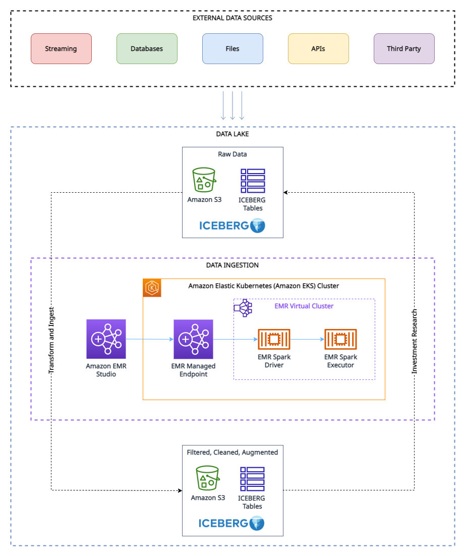
As shown in the architecture diagram, the research data lake is built on Amazon S3 and managed using Apache Iceberg, which is an open table format bringing the reliability and simplicity of relational database management service (RDBMS) tables to data lakes. To avoid look-ahead bias in backtesting, it’s essential to create snapshots of the data at different points in time. However, managing and organizing these snapshots can be challenging, especially when dealing with a large volume of data.

This is where the tagging feature in Apache Iceberg comes in handy. With tagging, researchers can create differently named snapshots of market data and track changes over time. For example, they can create a snapshot of the data at the end of each trading day and tag it with the date and any relevant market conditions.

By using tags to organize the snapshots, researchers can easily query and analyze the data based on specific market conditions or events, without having to worry about the specific dates of the data. This can be particularly helpful when conducting research that is not time-sensitive or when looking for trends over long periods of time.

Furthermore, the tagging feature can also help with other aspects of data management, such as data retention for GDPR compliance, and maintaining lineages of the table via different branches. Researchers can use Apache Iceberg tagging to ensure the integrity and accuracy of their data while also simplifying data management.

Prerequisites

To follow along with this walkthrough, you must have the following:

• An AWS account with an IAM role that has sufficient access to provision the required resources.
• To comply with licensing considerations, we cannot provide a sample of the ETF constituents data. Therefore, it must be purchased separately for the dataset onboarding purposes.

Solution overview

To set up and test this experiment, we complete the following high-level steps:

1. Create an S3 bucket.
2. Load the dataset into Amazon S3. For this post, the ETF data referred to was obtained via API call through a third-party provider, but you can also consider the following options:
   1. You can use the following prescriptive guidance, which describes how to automate data ingestion from various data providers into a data lake in Amazon S3 using AWS Data Exchange.
   2. You can also utilize AWS Data Exchange to select from a range of third-party dataset providers. It simplifies the usage of data files, tables, and APIs for your specific needs.
   3. Lastly, you can also refer to the following post on how to use AWS Data Exchange for Amazon S3 to access data from a provider bucket: Analyzing impact of regulatory reform on the stock market using AWS and Refinitiv data.
3. Create an EMR cluster. You can use this Getting Started with EMR tutorial or we used CDK to deploy an EMR on EKS environment with a custom managed endpoint.
4. Create an EMR notebook using EMR Studio. For our testing environment, we used a custom build Docker image, which contains Iceberg v1.3. For instructions on attaching a cluster to a Workspace, refer to Attach a cluster to a Workspace.
5. Configure a Spark session. You can follow along via the following sample notebook.
6. Create an Iceberg table and load the test data from Amazon S3 into the table.
7. Tag this data to preserve a snapshot of it.
8. Perform updates to our test data and tag the updated dataset.
9. Run simulated backtesting on our test data to find the most profitable entry point for a trade.

Create the experiment environment

We can get up and running with Iceberg by creating a table via Spark SQL from an existing view, as shown in the following code:

spark.sql("""
CREATE TABLE glue_catalog.quant.etf_holdings 
USING iceberg OPTIONS ('format-version'='2') 
LOCATION 's3://substitute_your_bucket/etf_holdings/' 
AS SELECT * FROM 2022Q1
""")
spark.sql("""
SELECT symbol, date, acceptanceTime, status
FROM glue_catalog.quant.etf_holdings
""").show()

+------+----------+-------------------+------+
|symbol|      date|     acceptanceTime|status|
+------+----------+-------------------+------+
|   HON|2022-03-31|2022-05-27 13:54:03|   new|
|   DFS|2022-03-31|2022-05-27 13:54:03|   new|
|   FMC|2022-03-31|2022-05-27 13:54:03|   new|
|  NDSN|2022-03-31|2022-05-27 13:54:03|   new|
|   CRL|2022-03-31|2022-05-27 13:54:03|   new|
|  EPAM|2022-03-31|2022-05-27 13:54:03|   new|
|  CSCO|2022-03-31|2022-05-27 13:54:03|   new|
|   ALB|2022-03-31|2022-05-27 13:54:03|   new|
|   AIZ|2022-03-31|2022-05-27 13:54:03|   new|
|   CRM|2022-03-31|2022-05-27 13:54:03|   new|
|  PENN|2022-03-31|2022-05-27 13:54:03|   new|
|  INTU|2022-03-31|2022-05-27 13:54:03|   new|
|   DOW|2022-03-31|2022-05-27 13:54:03|   new|
|   LHX|2022-03-31|2022-05-27 13:54:03|   new|
|   BLK|2022-03-31|2022-05-27 13:54:03|   new|
|  ZBRA|2022-03-31|2022-05-27 13:54:03|   new|
|   UPS|2022-03-31|2022-05-27 13:54:03|   new|
|    DG|2022-03-31|2022-05-27 13:54:03|   new|
|  DISH|2022-03-31|2022-05-27 13:54:03|   new|
|      |2022-03-31|2022-05-27 13:54:03|   new|
+------+----------+-------------------+------+

Now that we’ve created an Iceberg table, we can use it for investment research. One of the key features of Iceberg is its support for scalable data versioning. This means that we can easily track changes to our data and roll back to previous versions without making additional copies. Because this data gets updated periodically, we want to be able to create named snapshots of the data so that quant traders have easy access to consistent snapshots of data that have their own retention policy. In this case, let’s tag the dataset to indicate that it represents the ETF holdings data as of Q1 2022:

spark.sql("""
ALTER TABLE glue_catalog.quant.etf_holdings CREATE TAG Q1_2022
""")

As we move forward in time and new data becomes available by Q3, we may need to update existing datasets to reflect these changes. In the following example, we first use an UPDATE statement to mark the stocks as expired in the existing ETF holdings dataset. Then we use the MERGE INTO statement based on matching conditions such as ISIN code. If a match is not found between the existing dataset and the new dataset, the new data will be inserted as new records in the table and status code will be set to ‘new’ for these records. Similarly, if the existing dataset has stocks that are not present in the new dataset, those records will remain expired with a status code of ‘expired’. Finally, for records where a match is found, the data in the existing dataset will be updated with the data from the new dataset, and record will have an unchanged status code. With Iceberg’s support for efficient data versioning and transactional consistency, we can be confident that our data updates will be applied correctly and without data corruption.

spark.sql("""
UPDATE glue_catalog.quant.etf_holdings
SET status = 'expired'
""")
spark.sql("""
MERGE INTO glue_catalog.quant.etf_holdings t
USING (SELECT * FROM 2022Q3) s
ON t.isin = s.isin
WHEN MATCHED THEN
    UPDATE SET t.acceptanceTime = s.acceptanceTime,
               t.date = s.date,
               t.balance = s.balance,
               t.valUsd = s.valUsd,
               t.pctVal = s.pctVal,
               t.status = "unchanged"
WHEN NOT MATCHED THEN INSERT *
""")

Because we now have a new version of the data, we use Iceberg tagging to provide isolation for each new version of data. In this case, we tag this as Q3_2022 and allow quant traders and other users to work on this snapshot of the data without being affected by ongoing updates to the pipeline:

spark.sql("""
ALTER TABLE glue_catalog.quant.etf_holdings CREATE TAG Q3_2022""")

This makes it very easy to see which stocks are being added and deleted. We can use Iceberg’s time travel feature to read the data at a given quarterly tag. First, let’s look at which stocks are added to the index; these are the rows that are in the Q3 snapshot but not in the Q1 snapshot. Then we will look at which stocks are removed; these are the rows that are in the Q1 snapshot but not in the Q3 snapshot:

spark.sql("""
SELECT symbol, isin, acceptanceTime, date 
FROM glue_catalog.quant.etf_holdings 
AS OF ‘Q3_2022’ EXCEPT 
SELECT symbol, isin, acceptanceTime, date 
FROM glue_catalog.quant.etf_holdings 
AS OF ‘Q1_2022’
""").show()

+------+------------+-------------------+----------+
|symbol|        isin|     acceptanceTime|      date|
+------+------------+-------------------+----------+
|   CPT|US1331311027|2022-11-28 15:50:55|2022-09-30|
|  CSGP|US22160N1090|2022-11-28 15:50:55|2022-09-30|
|  EMBC|US29082K1051|2022-11-28 15:50:55|2022-09-30|
|  INVH|US46187W1071|2022-11-28 15:50:55|2022-09-30|
|     J|US46982L1089|2022-11-28 15:50:55|2022-09-30|
|   KDP|US49271V1008|2022-11-28 15:50:55|2022-09-30|
|    ON|US6821891057|2022-11-28 15:50:55|2022-09-30|
|  VICI|US9256521090|2022-11-28 15:50:55|2022-09-30|
|   WBD|US9344231041|2022-11-28 15:50:55|2022-09-30|
+------+------------+-------------------+----------+

spark.sql("""
SELECT symbol, isin, acceptanceTime, date 
FROM glue_catalog.quant.etf_holdings 
AS OF ‘Q1_2022’ EXCEPT 
SELECT symbol, isin, acceptanceTime, date 
FROM glue_catalog.quant.etf_holdings 
AS OF ‘Q3_2022’
""").show()

+------+------------+-------------------+----------+
|symbol|        isin|     acceptanceTime|      date|
+------+------------+-------------------+----------+
|  PENN|US7075691094|2022-05-27 13:54:03|2022-03-31|
|    UA|US9043112062|2022-05-27 13:54:03|2022-03-31|
|   UAA|US9043111072|2022-05-27 13:54:03|2022-03-31|
|   LTP|US7127041058|2022-05-27 13:54:03|2022-03-31|
| DISCA|US25470F1049|2022-05-27 13:54:03|2022-03-31|
|  CERN|US1567821046|2022-05-27 13:54:03|2022-03-31|
|  IPGP|US44980X1090|2022-05-27 13:54:03|2022-03-31|
|      |US25470F3029|2022-05-27 13:54:03|2022-03-31|
|     J|US4698141078|2022-05-27 13:54:03|2022-03-31|
|   PVH|US6936561009|2022-05-27 13:54:03|2022-03-31|
+------+------------+-------------------+----------+

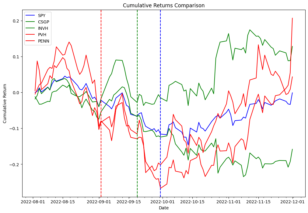
Now we use the delta obtained in the preceding code to backtest the following strategy. As part of the index rebalancing arbitrage process, we’re going to long stocks that are added to the index and short stocks that are removed from the index, and we’ll test this strategy for both the effective date and announcement date. As a proof of concept from the two different lists, we picked PVH and PENN as removed stocks, and CSGP and INVH as added stocks.

To follow along with the examples below, you will need to use the notebook provided in the Quant Research example GitHub repository.

import numpy as np
import vectorbt as vbt

def backtest(entry_point='2022-09-02', exit_point='2022-10-31'):
    open_position = (historical_prices_pd.index == entry_point)
    close_position = (historical_prices_pd.index == exit_point)

    CASH = 100000
    COMMPERC = 0.000

    symbol_cols = pd.Index(['PENN', 'PVH', 'INVH', 'CSGP'], name='symbol')
    order_size = pd.DataFrame(index=historical_prices_pd.index, columns=symbol_cols)
    order_size['PENN'] = np.nan
    order_size['PVH'] = np.nan
    order_size['INVH'] = np.nan
    order_size['CSGP'] = np.nan

    #short
    order_size.loc[open_position, 'PENN'] = -10
    order_size.loc[close_position, 'PENN'] = 0

    order_size.loc[open_position, 'PVH'] = -10
    order_size.loc[close_position, 'PVH'] = 0

    #long
    order_size.loc[open_position, 'INVH'] = 10
    order_size.loc[close_position, 'INVH'] = 0

    order_size.loc[open_position, 'CSGP'] = 10
    order_size.loc[close_position, 'CSGP'] = 0

    # Execute at the next bar
    order_size = order_size.vbt.fshift(1)

    portfolio = vbt.Portfolio.from_orders(
            historical_close_prices,  # current close as reference price
            size=order_size,  
            price=historical_open_prices,  # current open as execution price
            size_type='targetpercent', 
            val_price=historical_close_prices.vbt.fshift(1),  # previous close as group valuation price
            init_cash=CASH,
            allow_partial=False,
            fees=COMMPERC,
            direction='both',
            cash_sharing=True,  # share capital between assets in the same group
            group_by=True,  # all columns belong to the same group
            call_seq='auto',  # sell before buying
            freq='d'  # index frequency for annualization
    )
    return portfolio

portfolio = backtest('2022-09-02', '2022-10-31')

portfolio.orders.records_readable.head(20)

The following table represent the portfolio orders records:

Experimentation findings

The following table shows Sharpe Ratios for various holding periods and two different trade entry points: announcement and effective dates.

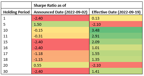
The data suggests that the effective date is the most profitable entry point across most holding periods, whereas the announcement date is an effective entry point for short-term holding periods (5 calendar days, 2 business days). Because the results are obtained from testing a single event, this is not statistically significant to accept or reject a hypothesis that index rebalancing events can be used to generate consistent alpha. The infrastructure we used for our testing can be used to run the same experiment required to do hypothesis testing at scale, but index constituents data is not readily available.

Conclusion

In this post, we demonstrated how the use of backtesting and the Apache Iceberg tagging feature can provide valuable insights into the performance of index arbitrage profitability strategies. By using a scalable Amazon EMR on Amazon EKS stack, researchers can easily handle the entire investment research lifecycle, from data collection to backtesting. Additionally, the Iceberg tagging feature can help address the challenge of look-ahead bias, while also providing benefits such as data retention control for GDPR compliance and maintaining lineage of the table via different branches. The experiment findings demonstrate the effectiveness of this approach in evaluating the performance of index arbitrage strategies and can serve as a useful guide for researchers in the finance industry.

About the Authors

Boris Litvin is Principal Solution Architect, responsible for financial services industry innovation. He is a former Quant and FinTech founder, and is passionate about systematic investing.

Guy Bachar is a Solutions Architect at AWS, based in New York. He accompanies greenfield customers and helps them get started on their cloud journey with AWS. He is passionate about identity, security, and unified communications.

Noam Ouaknine is a Technical Account Manager at AWS, and is based in Florida. He helps enterprise customers develop and achieve their long-term strategy through technical guidance and proactive planning.

Sercan Karaoglu is Senior Solutions Architect, specialized in capital markets. He is a former data engineer and passionate about quantitative investment research.

Jack Ye is a software engineer in the Athena Data Lake and Storage team. He is an Apache Iceberg Committer and PMC member.

Amogh Jahagirdar is a Software Engineer in the Athena Data Lake team. He is an Apache Iceberg Committer.