AWS Big Data Blog
Create a most-recent view of your data lake using Amazon Redshift Serverless
Building a robust data lake is very beneficial because it enables organizations have a holistic view of their business and empowers data-driven decisions. The curated layer of a data lake is able to hydrate multiple homogeneous data products, unlocking limitless capabilities to address current and future requirements. However, some concepts of how data lakes work feel counter-intuitive for professionals with a traditional database background.
Data lakes are by design append-only, meaning that the new records with an existing primary key don’t update the existing values out-of-the box; instead the new values are appended, resulting in having multiple occurrences of the same primary key in the data lake. Furthermore, special care needs to be taken to handle row deletions, and even if there is a way to identify deleted primary keys, it’s not straightforward to incorporate them to the data lake.
Traditionally, processing between the different layers of data lakes is performed using distributed processing engines such as Apache Spark that can be deployed in a managed or serverless way using services such as Amazon EMR or AWS Glue. Spark has recently introduced frameworks that give data lakes a flavor of ACID properties, such as Apache Hudi, Apache Iceberg, and Delta Lake. However, if you’re coming from a database background, there is a significant learning curve to adopt these technologies that involves understanding the concepts, moving away from SQL to a more general-purpose language, and adopting a specific ACID framework and its complexities.
In this post, we discuss how to implement a data lake that supports updates and deletions of individual rows using the Amazon Redshift ANSI SQL compliant syntax as our main processing language. We also take advantage of its serverless offering to address scenarios where consumption patterns don’t justify creating a managed Amazon Redshift cluster, which makes our solution cost-efficient. We use Python to interact with the AWS API, but you can also use any other AWS SDK. Finally, we use AWS Glue auto-generated code to ingest data to Amazon Redshift Serverless and AWS Glue crawlers to create metadata for our datasets.
Solution overview
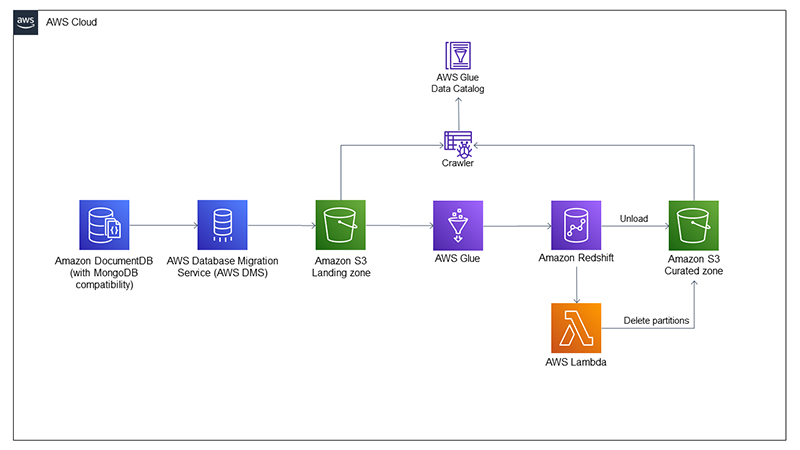
Most of the services we use for this post can be treated as placeholders. For instance, we use Amazon DocumentDB (with MongoDB compatibility) as our data source system, because one of the key features of a data lake is that it can support structured and unstructured data. We use AWS Database Migration Service (AWS DMS) to ingest data from Amazon DocumentDB to the data lake on Amazon Simple Storage Service (Amazon S3). The change data capture (CDC) capabilities of AWS Database Migration Service (AWS DMS) enable us to identify both updated and deleted rows that we want to propagate to the data lake. We use an AWS Glue job to load raw data to Redshift Serverless to use job bookmarks, which allows each run of the load job to ingest new data. You could replace the AWS Glue job with Amazon Redshift Spectrum or the Amazon Redshift COPY command if there is a different way to identify newly arrived data.
After new data is ingested to Amazon Redshift, we use it as our extract, transform, and load (ETL) engine. We trigger a stored procedure to curate the new data, upsert it to our existing table, and unload it to the data lake. To handle data deletions, we have created a scalar UDF in AWS Lambda that we can call from Amazon Redshift to delete the S3 partitions that have been affected by the newly ingested dataset before rewriting them with the updated values. The following diagram showcases the architecture of our solution.
Data ingestion
The dataset we use for this post is available on GitHub. After we create our Amazon DocumentDB instance (for this post, we used engine version 4.0.0 and the db.t3.medium instance class), we ingest the sample dataset. Ingested records look like the this:
We then create an AWS DMS dms.t3.medium instance using engine version 3.4.6, a source endpoint for Amazon DocumentDB, and a target endpoint for Amazon S3, adding dataFormat=parquet; as an extra configuration, so that records are stored in Parquet format in the landing zone of the data lake. After we confirm the connectivity of the endpoints using the Test connection feature, we create a database migration task for full load and ongoing replication. We can confirm data is migrated successfully to Amazon S3 by browsing in the S3 location and choosing Query with S3 Select on the Parquet file that has been generated. The result looks like the following screenshot.

We then catalog the ingested data using an AWS Glue crawler on the landing zone S3 bucket, so that we can query the data with Amazon Athena and process it with AWS Glue.
Set up Redshift Serverless
Amazon Redshift is a fully managed, petabyte-scale data warehouse service in the cloud. You can start with just a few hundred gigabytes of data and scale to a petabyte or more. This enables you to use your data to acquire new insights for your business and customers. It’s not uncommon to want to take advantage of the rich features Amazon Redshift provides without having a workload demanding enough to justify purchasing an Amazon Redshift provisioned cluster. To address such scenarios, we have launched Redshift Serverless, which includes all the features provisioned clusters have but enables you to only pay for the workloads you run rather than paying for the entire time your Amazon Redshift cluster is up.
Our next step is to set up our Redshift Serverless instance. On the Amazon Redshift console, we choose Redshift Serverless, select the required settings (similar to creating a provisioned Amazon Redshift cluster), and choose Save configuration. If you intend to access your Redshift Serverless instance via a JDBC client, you might need to enable public access. After the setup is complete, we can start using the Redshift Serverless endpoint.
Load data to Redshift Serverless
To confirm our serverless point is accessible, we can create an AWS Glue connection and test its connectivity. The type of the connection is JDBC, and we can find our serverless JDBC URL from the Workgroup configuration section on our Redshift Serverless console. For the connection to be successful, we need to configure the connectivity between the Amazon Redshift and AWS Glue security groups. For more details, refer to Connecting to a JDBC Data Store in a VPC. After connectivity is configured correctly, we can test the connection and if the test is successful, we should see the following message.

We use an AWS Glue job to load the historical dataset to Amazon Redshift; however, we don’t apply any business logic at this step because we want to implement our transformations using ANSI SQL in Amazon Redshift. Our AWS Glue job is mostly auto-generated boilerplate code:
The job reads the table cases from the database document_landing from our AWS Glue Data Catalog, created by the crawler after data ingestion. It copies the underlying data to the table cases_stage in the database dev of the cluster defined in the AWS Glue connection redshift-serverless. We can run this job and use the Amazon Redshift query editor v2 on the Amazon Redshift console to confirm its success by seeing the newly created table, as shown in the following screenshot.

We can now query and transform the historical data using Redshift Serverless.
Transform stored procedure
We have created a stored procedure that performs some common transformations, such as converting a text to date and extracting the year, month, and day from it, and creating some boolean flag fields. After the transformations are performed and stored to the cases table, we want to unload the data to our data lake S3 bucket and finally empty the cases_stage table, preparing it to receive the next CDC load of our pipeline. See the following code:
Note that for unloading data to Amazon S3, we need to create the AWS Identity and Access Management (IAM) role arn:aws:iam::<AWS account-id>:role/<role-name>, give it the required Amazon S3 permissions, and associate it with our Redshift Serverless instance. Calling the stored procedure after ingesting the historical dataset to the cases_stage table results in loading the transformed and partitioned dataset in the S3 folder specified in Parquet format. After we crawl the folder with an AWS Glue crawler, we can verify the results using Athena.

We can revisit the loading AWS Glue job we described before to automatically invoke the steps we triggered manually. We can use an Amazon Redshift postactions configuration to trigger the stored procedure as soon as the loading of the staging table is complete. We can also use Boto3 to trigger the AWS Glue crawler when data is unloaded to Amazon S3. Therefore, the revisited AWS Glue job looks like the following code:
CDC load
Because the AWS DMS migration task we configured is for full load and ongoing replication, it can capture updates and deletions on a record level. Updates come with an OP column with value U, such as in the following example:
Deletions have an OP column with value D, the primary key to be deleted, and all other fields empty:
Enabling job bookmarks for our AWS Glue job guarantees that subsequent runs of the job only process new data since the last checkpoint that was set in the previous run of the job without any changes in our code. After the CDC data is loaded in the staging table, our next step is to delete rows with OP column D, perform a merge operation to replace existing rows, and upload the result to our S3 bucket. However, because S3 objects are immutable, we need to delete the partitions that would be affected by the latest ingested dataset and rewrite them from Amazon Redshift. Amazon Redshift doesn’t have an out-of-the-box way to delete S3 objects; however, we can use a scalar Lambda UDF that takes as an argument the partition to be deleted and removes all the objects under the partition. The Python code of our Lambda function uses Boto3 and looks like the following example:
We then need to register the Lambda UDF from in our Amazon Redshift cluster by running the following code:
The last edge case we might need to take care of is the scenario of a CDC dataset containing multiple records for the same dataset. The approach we take here is to use another date field that is available in the dataset, prep_flow_time, to keep the latest record. To implement this logic in SQL, we use a nested query with the row_number window function.
On a high level, the upsert stored procedure includes the following steps:
- Delete partitions that are being updated from the S3 data lake, using the scalar Lambda UDF.
- Delete rows that are being updated from Amazon Redshift.
- Implement the transformations and compute the latest values of the updated rows.
- Insert them into the target table in Amazon Redshift.
- Unload the affected partitions to the S3 data lake.
- Truncate the staging table.
See the following code:
Finally, we can modify the aforementioned AWS Glue job to use Boto3 to decide whether this is a historical load or a CDC by using Boto3 to check if the table exists in the AWS Glue Data Catalog. The final version of the AWS Glue job is as follows:
Running this job for the first time with job bookmarks enabled loads the historical data to the Redshift Serverless staging table and triggers the historical load stored procedure, which in turn performs the transformations we implemented using SQL and unloads the result to the S3 data lake. Subsequent runs ingest newly arrived data from the landing zone, ingests them to the staging table, and performs the upsert process, deleting and repopulating the affected partitions in the data lake.
Conclusion
Building a modern data lake that maintains a most recent view involves some edge cases that aren’t intuitive if you come from a RDBMS background. In this post, we described an AWS native approach that takes advantage of the rich features and SQL syntax of Amazon Redshift, paying only for the resources used thanks to Redshift Serverless and without using any external framework.
The introduction of Amazon Redshift Serverless unlocks the hundreds of Redshift features released every year to users that do not require a cluster that’s always up and running. You can start experimenting with this approach of managing your data lake with Redshift, as well as addressing other use cases that are now easier to solve with Redshift Serverless.
About the author
 George Komninos is a solutions architect for the AWS Data Lab. He helps customers convert their ideas to a production-ready data product. Before AWS, he spent three years at Alexa Information domain as a data engineer. Outside of work, George is a football fan and supports the greatest team in the world, Olympiacos Piraeus.