AWS Big Data Blog
Install Python libraries on a running cluster with EMR Notebooks
May 2024: This post was reviewed and updated for accuracy.
Amazon EMR Studio is an integrated development environment (IDE) that provides fully managed Jupyter Notebooks and tools such as Spark UI and YARN Timeline Service.
This post discusses installing notebook-scoped libraries on a running cluster directly via an EMR Studio Workspace. Before this feature, you had to rely on bootstrap actions or use custom AMI to install additional libraries that are not pre-packaged with the EMR AMI when you provision the cluster. This post also discusses how to use the pre-installed Python libraries available locally within EMR Studio to analyze and plot your results. This capability is useful in scenarios in which you don’t have access to a PyPI repository but need to analyze and visualize a dataset.
For those interested in combining interactive data preparation and machine learning at scale within a single notebook, Amazon Web Services announced Amazon SageMaker Universal Notebooks at re:Invent 2021. Universal Notebooks allows data science teams to easily create and manage Amazon EMR clusters from Amazon SageMaker Studio to run interactive Spark and ML workloads.
Benefits of using notebook-scoped libraries with EMR Notebooks
Notebook-scoped libraries provide you the following benefits:
- Runtime installation – You can import your favorite Python libraries from PyPI repositories and install them on your remote cluster on the fly when you need them. These libraries are instantly available to your Spark runtime environment. There is no need to restart the notebook session or recreate your cluster.
- Dependency isolation – The libraries you install using EMR Studio are isolated to your notebook session and don’t interfere with bootstrapped cluster libraries or libraries installed from other notebook sessions. These notebook-scoped libraries take precedence over bootstrapped libraries. Multiple notebook users can import their preferred version of the library and use it without dependency clashes on the same cluster.
- Portable library environment – The library package installation happens from your notebook file. This allows you to recreate the library environment when you switch the notebook to a different cluster by re-executing the notebook code. At the end of the notebook session, the libraries you install through EMR Studio are automatically removed from the hosting EMR cluster.
Prerequisites
To use this feature in EMR Studio, you need a Workspace attached to a cluster running EMR release 5.26.0 or later. The cluster should have access to the public or private PyPI repository from which you want to import the libraries. For more information, see Use an Amazon EMR Studio.
There are different ways to configure your VPC networking to allow clusters inside the VPC to connect to an external repository. For more information, see Scenarios and Examples in the Amazon VPC User Guide.
Using notebook-scoped libraries
This post demonstrates the notebook-scoped libraries feature of EMR Studio by analyzing the Amazon shopping queries dataset. For more information, see amazon-science/esci-data on GitHub.
Open your workspace, select a notebook, and make sure the kernel is set to PySpark. Run the following command from the notebook cell:
You get the following output:

You can examine the current notebook session configuration by running the following command:
The notebook session is configured for Python 3 by default (through spark.pyspark.python). If you prefer to use Python 2, reconfigure your notebook session by running the following command from your notebook cell:
Before starting your analysis, check the libraries that are already available on the cluster. You can do this using the list_packages() PySpark API, which lists all the Python libraries on the cluster. Run the following code:
The first step is to copy the publicly available Amazon Science GSCI dataset from GitHub to an Amazon S3 bucket that is accessible by your EMR cluster. For more information, see How to get data into Amazon EMR.
After copying the Amazon Science GSCI dataset to Amazon S3, load the Amazon shopping queries dataset into a Spark DataFrame with the following code:
You are now ready to explore the data. Determine the schema and number of available columns in your dataset with the following code:
The following code is the output:
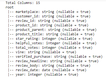
This dataset has a total of 15 columns. You can also check the total rows in your dataset by running the following code:
You get the following output:

Check the total number of books with the following code:
You get the following output:

You can also analyze the number of book reviews by year and find the distribution of customer ratings. To do this, import the Pandas library version 0.25.1 and the latest Matplotlib library from the public PyPI repository. Install them on the cluster attached to your notebook using the install_pypi_package API. See the following code:
You get the following output:

The install_pypi_package PySpark API installs your libraries along with any associated dependencies. By default, it installs the latest version of the library that is compatible with the Python version you are using. You can also install a specific version of the library by specifying the library version from the previous Pandas example.
Verify that your imported packages successfully installed by running the following code:
You can also analyze the trend for the number of reviews provided across multiple years. Use ‘toPandas()’ to convert the Spark data frame to a Pandas data frame, which you can visualize with Matplotlib. See the following code:
The preceding commands render the plot on the attached EMR cluster. To visualize the plot within your notebook, use %matplot magic. See the following code:
The generated chart shows that the number of products skews towards the us locale with almost three-quarters of the representation.

You can also analyze the distribution of ESCI labels and visualize it using a pie chart. See the following code:
Print the pie chart using %matplot magic and visualize it from your notebook with the following code:
The generated chart shows that our dataset skews towards the I ESCI label, which stands for “Irrelevant”. Approximately 70% of our dataset’s product responses are irrelevant to the initial query. Conversely, approximately 5% of our dataset’s product responses are an exact match to the initial query.
Lastly, use the ‘uninstall_package’ Pyspark API to uninstall the Pandas library that you installed using the install_package API. This is useful in scenarios in which you want to use a different version of a library that you previously installed using EMR Notebooks. See the following code:
Next, run the following code:
After closing your notebook, the Pandas and Matplot libraries that you installed on the cluster using the install_pypi_package API are garbage and collected out of the cluster.
Using local Python libraries in EMR Notebooks
The notebook-scoped libraries discussed previously require your EMR cluster to have access to a PyPI repository. If you cannot connect your EMR cluster to a repository, use the Python libraries pre-packaged with EMR Notebooks to analyze and visualize your results locally within the notebook. Unlike the notebook-scoped libraries, these local libraries are only available to the Python kernel and are not available to the Spark environment on the cluster. To use these local libraries, export your results from your Spark driver on the cluster to your notebook and use the notebook magic to plot your results locally. Because you are using the notebook and not the cluster to analyze and render your plots, the dataset that you export to the notebook has to be small (recommend less than 100 MB).
To see the list of local libraries, run the following command from the notebook cell:
You get a list of all the libraries available in the notebook. Because the list is rather long, this post doesn’t include them.
For this analysis, find out the top 10 most frequent products from your shopping queries dataset and analyze the ESCI label distribution for these products.
You can identify the children’s books by using customers’ written reviews with the following code:
Plot the top 10 children’s books by number of customer reviews with the following code:
Analyze the ESCI label distribution for these products with the following code:
To plot these results locally within your notebook, export the data from the Spark driver and cache it in your local notebook as a Pandas DataFrame. To achieve this, first register a temporary table with the following code:
Use the local SQL magic to extract the data from this table with the following code:
For more information about these magic commands, see the GitHub repo.
After you execute the code, you get a user-interface to interactively plot your results. The following pie chart shows the ESCI distribution for the top 10 products:

You can also plot more complex charts by using local Matplot and seaborn libraries available with EMR Notebooks. See the following code:
You get the following output:

Summary
This post showed how to use the notebook-scoped libraries feature of EMR Studio to import and install your favorite Python libraries at runtime on your EMR cluster, and use these libraries to enhance your data analysis and visualize your results in rich graphical plots. The post also demonstrated how to use the pre-packaged local Python libraries available in EMR Studio to analyze and plot your results.
About the Authors
 Parag Chaudhari is a Software Development Engineer at AWS.
 Ethan Pritchard is a Software Development Engineer at AWS.
Audit History
Last reviewed and updated in April 2024 by Ethan Pritchard | Software Dev Engineer