AWS Big Data Blog
Building a cost efficient, petabyte-scale lake house with Amazon S3 lifecycle rules and Amazon Redshift Spectrum: Part 2
In part 1 of this series, we demonstrated building an end-to-end data lifecycle management system integrated with a data lake house implemented on Amazon Simple Storage Service (Amazon S3) with Amazon Redshift and Amazon Redshift Spectrum. In this post, we address the ongoing operation of the solution we built.
Data ageing process after a month (ongoing)
Let’s assume a month has elapsed since walking through the use case in the last post, and old historical data was classified and tiered accordingly to policy. You now need to enter the new monthly data generated into the lifecycle pipeline as follows:
- June 2020 data – Produced and consolidated into Amazon Redshift local tables
- December 2019 data – Migrated to Amazon S3
- June 2019 data – Migrated from Amazon S3 to S3-IA
- March 2019 data – Migrated from S3-IA to Glacier
The first step required is to increase the ageing counter of all the Parquet files (both midterm and shortterm prefixes), using aws s3api get-object-tagging to check the current value and increasing by 1 with aws s3api set-object-tagging. This can be cumbersome if you have many objects, but you can automate it with Amazon S3 CLI scripts or SDKs like Boto3 (Phyton).
The following is a simple Python script you can use to check the current tag settings for all keys in the prefix extract_shortterm:
This second Python script lists all current tag settings for all keys in the prefix extract_shortterm, increases by 1 ageing, and lists the keys and new tag values. If other tags were added to these objects prior to this step, this new tag overwrites the entire tagSet. The set object tagging operation is not an append, but a completely new PUT.
To run the pipeline described before, you need to perform the following:
- Unload the December 2019 data.
- Apply the tag
ageingto 6. - Add the new Parquet file as a new partition to the external table
taxispectrum.taxi_archive.
For the relevant syntax, see [part 1]. You can automate these tasks using an AWS Lambda function and use a monthly schedule.
Check the results with a query to the external table and don’t forget to remove unloaded items from the Amazon Redshift local table, as you did in part 1 of this series.
In this use case, we know exactly the mapping of June 2019 to the Amazon S3 key name because we used a specific naming convention. If your use case is different, you can use the two pseudo-columns automatically created in every Amazon Redshift external table: $path and $size. See the following code:
The following screenshot shows our results.

We’re migrating the March 2019 Parquet file to Glacier, so you should remove the related partition from the AWS Glue Data Catalog:
Right to be forgotten
One of the pillar rules of GDPR is the “right to be forgotten” rule—the ability for a customer or employee to request deletion of any personal data.
Implementing this feature for external tables on Amazon Redshift requires a different approach than for local tables, because external tables don’t support delete and update operations.
You can implement two different approaches.
In and out
In this first approach, you copy the external table to a temporary Amazon Redshift table, delete the specific rows, unload the temporary table to Amazon S3 and overwrite the key name, and drop the temporary (internal table).
Let’s assume that the drivers in the dataset are identified with column pulocid. We want to delete all records related to a driver identified with pulocid 129 and who worked between October 2019 and November 2019.
- With the following code (from Amazon Redshift), you can identify a every single row matched with specific single Parquet file:
The following screenshot shows our results.

- When checking the applied tags, note the value associated to the
ageingtag, or save the output of the following command in a temporary JSON file: - Create two temporary tables, one for each of the two Parquet files matching the query (October and November):
- Copy the Parquet file to the local table, using the format as parquet attribute:
- Delete the records matching the “right to be forgotten” request criteria:
- Overwrite the Parquet file with the UNLOAD command (note the
allowoverwriteoption): - Drop the temporary table:
In more complex use cases, user data might span multiple months, and our approach might not be effective. In these cases, using Spark to process and rewrite the Parquet could be a better and faster solution.
In other use cases, the number of records to be deleted could be a majority. If so, as an alternative to the delete and unload steps, you could use CREATE EXTERNAL TABLE AS (CTAS). CTAS creates an external table based on the column definition from a query and writes the results of that query on Amazon S3.
Edit your own
The second option is to use an external editor to access the Amazon S3 file and remove specific records. You could use a Spark script with the following steps:
- Create a DataFrame.
- Import a Parquet file in memory.
- Remove records matching your criteria.
- Overwrite the same Amazon S3 key with the new data.
Building a simple data ageing dashboard
Sometimes data temperature is very predictable and based on ageing, but in some cases, especially when data is originated and accessed from different entities, it’s not easy to build a model to fit the best storage transition strategy. For these scenarios, you can use Amazon S3 analytics storage class analysis and Amazon S3 access logs.
Storage class analytis observes the infrequent access patterns of a filtered set of data over a period of time. You can use the analysis results to help you improve your lifecycle policies. You can configure storage class analysis to analyze all the objects in a bucket rr, and configure filters to group objects together for analysis by a common prefix (objects that have names that begin with a common string), by object tags, or by both prefix and tags. Filtering by object groups is the best way to benefit from storage class analysis.
To achieve a better understanding of how data is accessed (and who accessed it, and when) and build a custom tiering strategy, you can use Amazon S3 access logs. This feature doesn’t have any additional costs, but log retention incurs Amazon S3 storage costs. You first define a recipient to store the logs.
- Create a new bucket named
rs-lakehouse-blog-post-logs. - To set up S3 Server access logging on the source bucket
rs-lakehouse-blog-poston the Amazon S3 console, on the Properties tab, choose Server access logging. - For Target bucket, enter
rs-lakehouse-blog-post-logs. - For Target prefix, leave blank.
- Choose Save.

Let’s assume that after few days of activities, you want to discover how users and applications accessed the data.
- On the Amazon Redshift console, create an external table to map the Amazon S3 access logs:
- Check the AWS Identity and Access Management (IAM) policy
S3-Lakehouse-Policycreated in part 1 and add the following two lines to the JSON definition file: - Query a few columns:
The following screenshot shows our results.
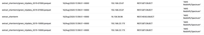
This report is a starting point for both auditing purposes and for analyzing access patterns. As a next step, you could use a business intelligence (BI) visualization solution like Amazon QuickSight and create a dataset in order to create a dashboard showing the most and least accessed files.
Cleaning up
To clean up your resources after walking through this post, complete the following steps:
- Delete the Amazon Redshift cluster without the final cluster snapshot:
- Delete the schema and table defined in AWS Glue:
- Delete the S3 buckets and all their content:
Conclusion
In the first post in this series, we demonstrated how to implement a data lifecycle system for a lake house using Amazon Redshift, Redshift Spectrum, and Amazon S3 lifecycle rules. In this post, we focused on how to operationalize the solution with automation scripts (with the AWS Boto3 library for Python) and S3 Server access logs.
About the Authors
 Cristian Gavazzeni is a senior solution architect at Amazon Web Services. He has more than 20 years of experience as a pre-sales consultant focusing on Data Management, Infrastructure and Security. During his spare time he likes eating Japanese food and travelling abroad with only fly and drive bookings.
 Francesco Marelli is a senior solutions architect at Amazon Web Services. He has lived and worked in London for 10 years, after that he has worked in Italy, Switzerland and other countries in EMEA. He is specialized in the design and implementation of Analytics, Data Management and Big Data systems, mainly for Enterprise and FSI customers. Francesco also has a strong experience in systems integration and design and implementation of web applications. He loves sharing his professional knowledge, collecting vinyl records and playing bass.