AWS Big Data Blog
Querying OpenStreetMap with Amazon Athena
This is a guest post by Seth Fitzsimmons, member of the 2017 OpenStreetMap US board of directors. Seth works with clients including the Humanitarian OpenStreetMap Team, Mapzen, the American Red Cross, and World Bank to craft innovative geospatial solutions.
OpenStreetMap (OSM) is a free, editable map of the world, created and maintained by volunteers and available for use under an open license. Companies and non-profits like Mapbox, Foursquare, Mapzen, the World Bank, the American Red Cross and others use OSM to provide maps, directions, and geographic context to users around the world.
In the 12 years of OSM’s existence, editors have created and modified several billion features (physical things on the ground like roads or buildings). The main PostgreSQL database that powers the OSM editing interface is now over 2TB and includes historical data going back to 2007. As new users join the open mapping community, more and more valuable data is being added to OpenStreetMap, requiring increasingly powerful tools, interfaces, and approaches to explore its vastness.
This post explains how anyone can use Amazon Athena to quickly query publicly available OSM data stored in Amazon S3 (updated weekly) as an AWS Public Dataset. Imagine that you work for an NGO interested in improving knowledge of and access to health centers in Africa. You might want to know what’s already been mapped, to facilitate the production of maps of surrounding villages, and to determine where infrastructure investments are likely to be most effective.
Note: If you run all the queries in this post, you will be charged approximately $1 based on the number of bytes scanned. All queries used in this post can be found in this GitHub gist.
What is OpenStreetMap?
As an open content project, regular OSM data archives are made available to the public via planet.openstreetmap.org in a few different formats (XML, PBF). This includes both snapshots of the current state of data in OSM as well as historical archives.
Working with “the planet” (as the data archives are referred to) can be unwieldy. Because it contains data spanning the entire world, the size of a single archive is on the order of 50 GB. The format is bespoke and extremely specific to OSM. The data is incredibly rich, interesting, and useful, but the size, format, and tooling can often make it very difficult to even start the process of asking complex questions.
Heavy users of OSM data typically download the raw data and import it into their own systems, tailored for their individual use cases, such as map rendering, driving directions, or general analysis. Now that OSM data is available in the Apache ORC format on Amazon S3, it’s possible to query the data using Athena without even downloading it.
How does Athena help?
You can use Athena along with data made publicly available via OSM on AWS. You don’t have to learn how to install, configure, and populate your own server instances and go through multiple steps to download and transform the data into a queryable form. Thanks to AWS and partners, a regularly updated copy of the planet file (available within hours of OSM’s weekly publishing schedule) is hosted on S3 and made available in a format that lends itself to efficient querying using Athena.
Asking questions with Athena involves registering the OSM planet file as a table and making SQL queries. That’s it. Nothing to download, nothing to configure, nothing to ingest. Athena distributes your queries and returns answers within seconds, even while querying over 9 years and billions of OSM elements.
You’re in control. S3 provides high availability for the data and Athena charges you per TB of data scanned. Plus, we’ve gone through the trouble of keeping scanning charges as small as possible by transcoding OSM’s bespoke format as ORC. All the hard work of transforming the data into something highly queryable and making it publicly available is done; you just need to bring some questions.
Registering Tables
The OSM Public Datasets consist of three tables:
- planet
Contains the current versions of all elements present in OSM. - planet_history
Contains a historical record of all versions of all elements (even those that have been deleted). - changesets
Contains information about changesets in which elements were modified (and which have a foreign key relationship to both the planet and planet_history tables).
To register the OSM Public Datasets within your AWS account so you can query them, open the Athena console (make sure you are using the us-east-1 region) to paste and execute the following table definitions:
planet
planet_history
changesets

Under the Hood: Extract, Transform, Load
So, what happens behind the scenes to make this easier for you? In a nutshell, the data is transcoded from the OSM PBF format into Apache ORC.
There’s an AWS Lambda function (running every 15 minutes, triggered by CloudWatch Events) that watches planet.openstreetmap.org for the presence of weekly updates (using rsync). If that function detects that a new version has become available, it submits a set of AWS Batch jobs to mirror, transcode, and place it as the “latest” version. Code for this is available at osm-pds-pipelines GitHub repo.
To facilitate the transcoding into a format appropriate for Athena, we have produced an open source tool, OSM2ORC. The tool also includes an Osmosis plugin that can be used with complex filtering pipelines and outputs an ORC file that can be uploaded to S3 for use with Athena, or used locally with other tools from the Hadoop ecosystem.
What types of questions can OpenStreetMap answer?
There are many uses for OpenStreetMap data; here are three major ones and how they may be addressed using Athena.
Case Study 1: Finding Local Health Centers in West Africa
When the American Red Cross mapped more than 7,000 communities in West Africa in areas affected by the Ebola epidemic as part of the Missing Maps effort, they found themselves in a position where collecting a wide variety of data was both important and incredibly beneficial for others. Accurate maps play a critical role in understanding human communities, especially for populations at risk. The lack of detailed maps for West Africa posed a problem during the 2014 Ebola crisis, so collecting and producing data around the world has the potential to improve disaster responses in the future.
As part of the data collection, volunteers collected locations and information about local health centers, something that will facilitate treatment in future crises (and, more importantly, on a day-to-day basis). Combined with information about access to markets and clean drinking water and historical experiences with natural disasters, this data was used to create a vulnerability index to select communities for detailed mapping.
For this example, you find all health centers in West Africa (many of which were mapped as part of Missing Maps efforts). This is something that healthsites.io does for the public (worldwide and editable, based on OSM data), but you’re working with the raw data.
Here’s a query to fetch information about all health centers, tagged as nodes (points), in Guinea, Sierra Leone, and Liberia:
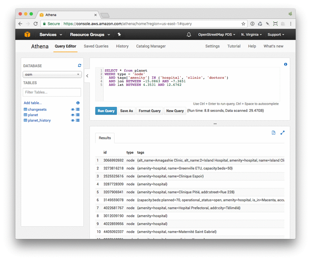
Buildings, as “ways” (polygons, in this case) assembled from constituent nodes (points), can also be tagged as medical facilities. In order to find those, you need to reassemble geometries. Here you’re taking the average of all nodes that make up a building (which will be the approximate center point, which is close enough for this purpose). Here is a query that finds both buildings and points that are tagged as medical facilities:

You could go a step further and query for additional tags included with these (for example, opening_hours) and use that as a metric for measuring “completeness” of the dataset and to focus on additional data to collect (and locations to fill out).
Case Study 2: Generating statistics about mapathons
OSM has a history of holding mapping parties. Mapping parties are events where interested people get together and wander around outside, gathering and improving information about sites (and sights) that they pass. Another form of mapping party is the mapathon, which brings together armchair and desk mappers to focus on improving data in another part of the world.
Mapathons are a popular way of enlisting volunteers for Missing Maps, a collaboration between many NGOs, education institutions, and civil society groups that aims to map the most vulnerable places in the developing world to support international and local NGOs and individuals. One common way that volunteers participate is to trace buildings and roads from aerial imagery, providing baseline data that can later be verified by Missing Maps staff and volunteers working in the areas being mapped.
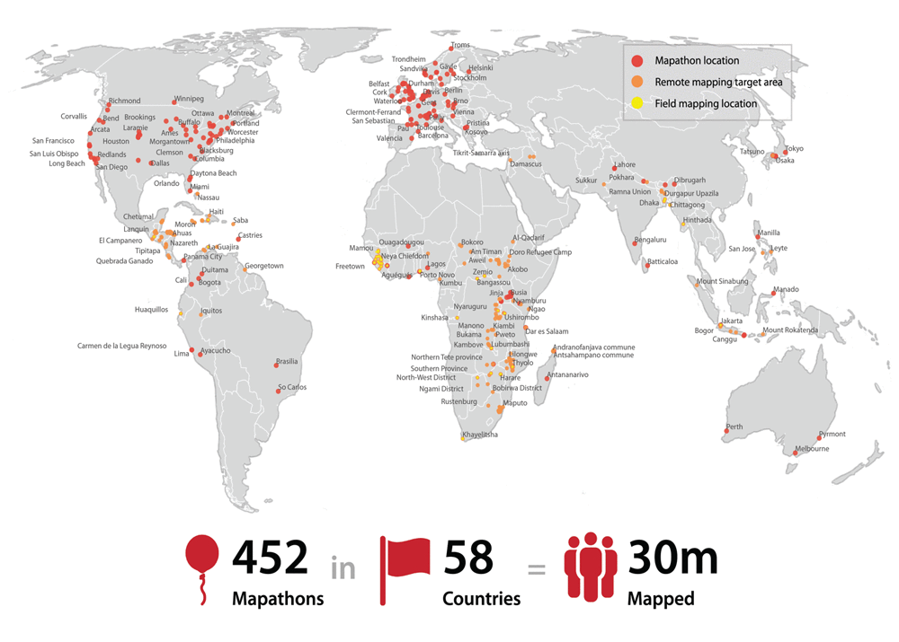
(Image and data from the American Red Cross)
Data collected during these events lends itself to a couple different types of questions. People like competition, so Missing Maps has developed a set of leaderboards that allow people to see where they stand relative to other mappers and how different groups compare. To facilitate this, hashtags (such as #missingmaps) are included in OSM changeset comments. To do similar ad hoc analysis, you need to query the list of changesets, filter by the presence of certain hashtags in the comments, and group things by username.
Now, find changes made during Missing Maps mapathons at George Mason University (using the #gmu hashtag):
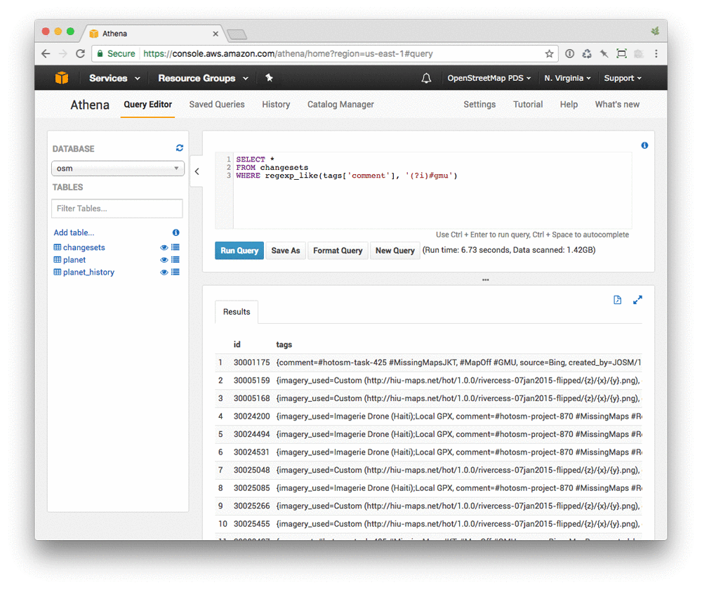
This includes all tags associated with a changeset, which typically include a mapper-provided comment about the changes made (often with additional hashtags corresponding to OSM Tasking Manager projects) as well as information about the editor used, imagery referenced, etc.
If you’re interested in the number of individual users who have mapped as part of the Missing Maps project, you can write a query such as:

25,610 people (as of this writing)!
Back at GMU, you’d like to know who the most prolific mappers are:

Nice job, BrokenString!
It’s also interesting to see what types of features were added or changed. You can do that by using a JOIN between the changesets and planet tables:

Using this as a starting point, you could break down the types of features, highlight popular parts of the world, or do something entirely different.
Case Study 3: Building Condition
With building outlines having been produced by mappers around (and across) the world, local Missing Maps volunteers (often from local Red Cross / Red Crescent societies) go around with Android phones running OpenDataKit and OpenMapKit to verify that the buildings in question actually exist and to add additional information about them, such as the number of stories, use (residential, commercial, etc.), material, and condition.
This data can be used in many ways: it can provide local geographic context (by being included in map source data) as well as facilitate investment by development agencies such as the World Bank.
Here are a collection of buildings mapped in Dhaka, Bangladesh:
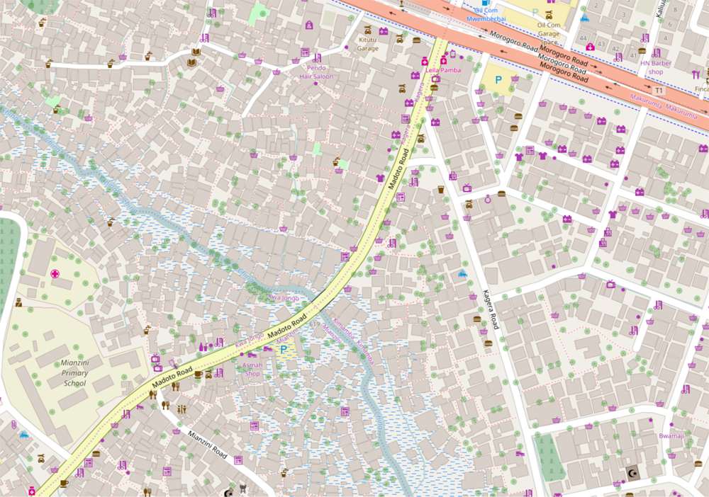
(Map and data © OpenStreetMap contributors)
For NGO staff to determine resource allocation, it can be helpful to enumerate and show buildings in varying conditions. Building conditions within an area can be a means of understanding where to focus future investments.
Querying for buildings is a bit more complicated than working with points or changesets. Of the three core OSM element types—node, way, and relation, only nodes (points) have geographic information associated with them. Ways (lines or polygons) are composed of nodes and inherit vertices from them. This means that ways must be reconstituted in order to effectively query by bounding box.
This results in a fairly complex query. You’ll notice that this is similar to the query used to find buildings tagged as medical facilities above. Here you’re counting buildings in Dhaka according to building condition:

Most buildings are unsurveyed (125,000 is a lot!), but of those that have been, most are average (as you’d expect). If you were to further group these buildings geographically, you’d have a starting point to determine which areas of Dhaka might benefit the most.
Conclusion
OSM data, while incredibly rich and valuable, can be difficult to work with, due to both its size and its data model. In addition to the time spent downloading large files to work with locally, time is spent installing and configuring tools and converting the data into more queryable formats. We think Amazon Athena combined with the ORC version of the planet file, updated on a weekly basis, is an extremely powerful and cost-effective combination. This allows anyone to start querying billions of records with simple SQL in no time, giving you the chance to focus on the analysis, not the infrastructure.
To download the data and experiment with it using other tools, the latest OSM ORC-formatted file is available via OSM on AWS at s3://osm-pds/planet/planet-latest.orc, s3://osm-pds/planet-history/history-latest.orc, and s3://osm-pds/changesets/changesets-latest.orc.
We look forward to hearing what you find out!