Advertising click-prediction modeling on Amazon EKS

In digital advertising, the ad click-through rate (CTR) model predicts the probability of a click given the ads and context x (for example, shopping query, time of the day, device). The output of a CTR model can be seen as a conditional probability p(y = click|x). A precise estimation of this probability influences our ability to optimally price ads for advertisers, drive customer engagement, and place ads in the right position.

Recently, there are neural network architectures that make use of feature embedding techniques. In Deep Interest Network for Click-Through Rate Prediction, most of these models adopt embedding followed by a multi-layer perceptron (MLP) with explicit or implicit feature interactions defined by the neural network architecture.

Our Amazon Advertising team works with big data and deep learning to model CTR predictions and bring relevant ads to delight our customers. We deal every day with datasets at petabyte scale and mine insights from data to improve predictions. The work requires us to be able to quickly analyze and process large datasets and the solution we use must easily scale to a large team of scientists and engineers.

In this blog post, we will use ad CTR prediction to introduce Amazon Elastic Kubernetes Service (Amazon EKS) as a compute infrastructure for big data workloads.

A typical solution

We use Apache Spark to process the datasets. Spark has been the leading framework in the big data ecosystem for years. It’s used by many production systems and can easily handle petabyte-scale datasets. Spark has many built-in libraries to efficiently build machine learning applications (for example, Spark MLLib, Spark Steaming, Spark SQL, and Spark GraphX). Our compute infrastructure for Spark is running on Amazon EMR, a service for automating Spark cluster lifecycle management for customers. Our team runs many ad-hoc and production jobs on Amazon EMR.

Going agile with Amazon EKS

Kubernetes is the industry-leading container orchestration engine. It provides powerful abstractions for managing all kinds of application deployment patterns, optimizing resource utilizations, and building agile, consistent environments in the application development process.

It’s natural to ask if we can run big data workloads on Kubernetes. It’s been discussed in AWS blog posts like Deploying Spark jobs on Amazon EKS and Optimizing Spark performance on Kubernetes. We think running some of our Spark applications on Kubernetes can greatly improve our engineering agility.

These are our requirements for a solution built with Amazon EKS:

• Agile: Users can start a Spark cluster and run applications in under a minute.
• Minimal configuration
• Autoscaling: Upon user request, compute resources must be allocated automatically.
• Multi-tenant: A large team of users must be able to run applications simultaneously without interfering with each other’s applications.

Architecture

The following figure shows the architecture of our solution. To run Jupyter notebook on EKS, we build Docker images that include Jupyter, Spark, and any required libraries. For information about how to build docker/jupyter/Dockerfile and docker/spark/Dockerfile, see the README on GitHub. Developers create a Jupyter notebook server as a pod in an Amazon EKS cluster. We set up a K8s service to front the pod deployment. Finally, we can use kubectl port-forward to set up a local connection to the Jupyter server and work on the notebooks locally.

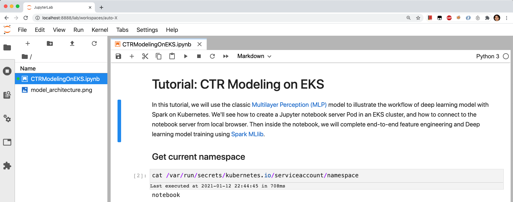
Tutorial: CTR modeling on Amazon EKS

In this tutorial, we will use the classic MLP model to illustrate the workflow of deep learning modeling running Spark on Kubernetes. We show how to create a Jupyter notebook server pod in an Amazon EKS cluster, how to connect to the notebook server from a local browser, and then from inside the notebook, we do end-to-end feature engineering and deep learning model training in Amazon EKS.

Clone the repository

To clone the repository, run git clone https://github.com/aws-samples/eks-ctr-modeling-example-using-spark.git.

In this tutorial, we assume that you’re running an Amazon EKS cluster. If you do not already have a cluster, follow the steps in Getting started with Amazon EKS to create one. Your cluster should have at least one node group backed by Amazon Elastic Compute Cloud (Amazon EC2) instances that have at least 4 cores and 20 GB of memory. For more information, see Amazon EC2 Instance Types. Enable Cluster Autoscaler to automatically adjust the number of nodes in your cluster as you spin up Spark drivers and executors.

Create namespace

First, create a namespace called notebook. For YAML files and information about how to create a namespace, roles, service account, deployment, and service, see the README on GitHub.

Create Spark ServiceAccount

Next, create a ClusterRoleBinding and ServiceAccount, which you will use to run Spark on Kubernetes.

Build Docker images

Note: Before you run the following commands, update the AWS_ACCOUNT_ID, REGION, and ECR-REPO.

The following image can be used as spark.kubernetes.container.image later in the tutorial notebook.

The following image can be used in jupyter-notebook.yaml.

Create Jupyter notebook server

Edit jupyter-notebook.yaml and replace the <REPLACE_WITH_JUPYTER_DOCKER_IMG> with the $JUPYTER_IMAGE you just built. Now run the notebook server as a Kubernetes deployment and build a service on it to expose IP addresses for the notebook UI and Spark UI.

To check the status of your service:

After your service is running, you can access the Jupyter notebook through port forwarding and open http://localhost:8888/lab.

It’s surprisingly fast to start a Spark cluster in Amazon EKS. You can start hundreds of executors in less than a minute depending on the availability of EC2 instances. This is a great time-saving feature that enables rapid data analysis. To make Spark available in your Jupyter notebook, you can use findspark to initialize and import PySpark just as regular libraries. You’ll be using the following library to create your Spark session with CPU, memory, Spark Shuffle partitions, and so on. The Kubernetes scheduler assigns the Spark executor containers to run as pods on the EC2 instances in an Amazon EKS cluster.

Create a notebook

In the file browser, click the + button and then in the Launcher tab, select the Python kernel. You can also start with the CTRModelingOnEKS.ipynb.

Note: Use the Spark Docker image you built earlier as the value of spark.kubernetes.container.image.

Sampling

At Amazon, we deal with petabyte-scale datasets. For the purpose of the tutorial, we synthesized two sample datasets to illustrate the workflow rather than the scale. We first load a small dataset with 100,000 rows to do feature engineering, model training, and so on. Later, we use a larger dataset with around one billion rows for execution. For information about how to create synthetic datasets in Spark, see GitHub notebook.

Feature engineering

Machine learning models expect numeric inputs in order to make predictions, but datasets usually come in an unstructured format. Because using the right numeric representation of features is crucial for the success of a machine learning model, we usually spend a lot of time understanding the data and applying appropriate transformations to the raw data to produce high-quality features. This process is called feature engineering. We cover a few common feature types and their associated feature engineering APIs in PySpark.

There are ten numerical features and one categorical feature in this raw dataset. Click is the label column. For simplicity, we use names like numeric_n for features. A quick exploratory data analysis (EDA) can show the ratio of click vs. non-click impressions in this dataset. As the following screenshot shows, there are 13,536 click impressions and 86,464 non-click impressions in this sample dataset.

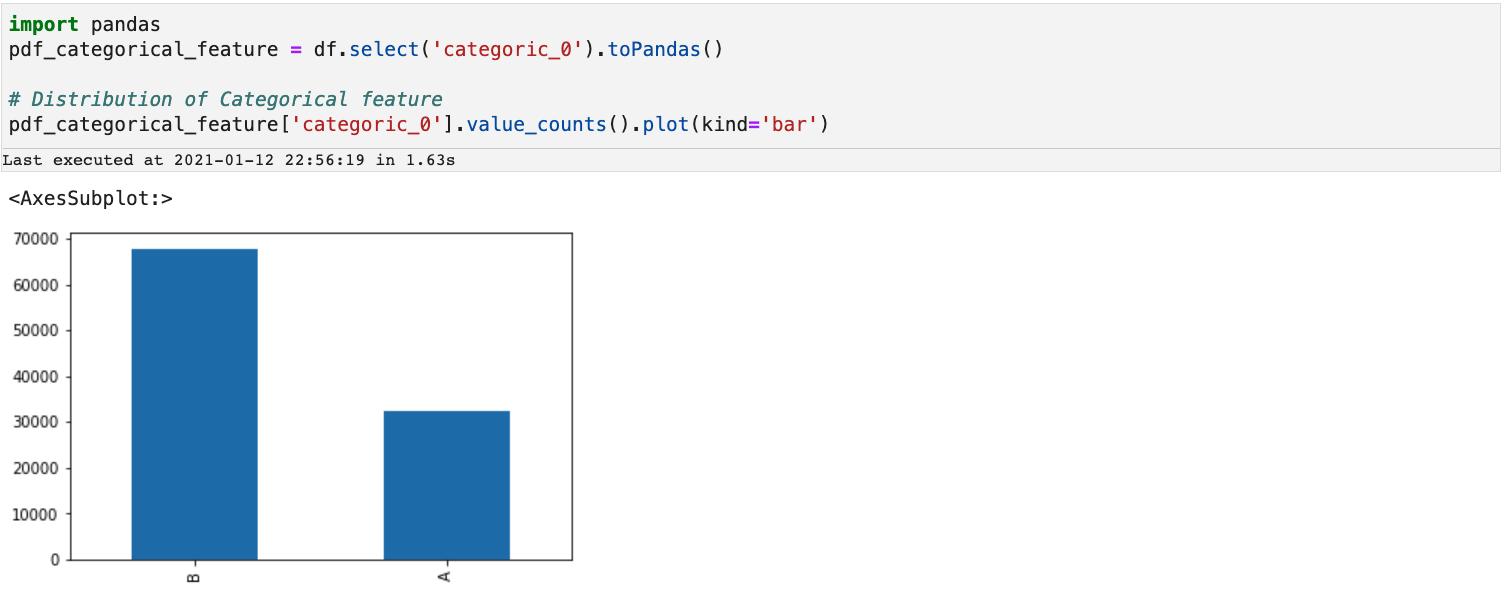
Categorical features

Categorical data is the most common type of data. The values are discrete and form a finite set. A typical example is the size of shirts. The values include S, M, L, XL, and so on. Feature engineering for categorical data applies transformations on the discrete values to produce distinct numeric values.

Here is a simple example of how we can achieve that with StringIndexer from PySpark.

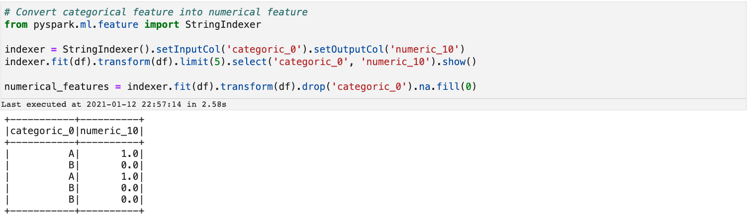As the output shows, StringIndexer maps B in column categoric_0 to 0.0 in column numeric_10 and A to 1.0.

Vectorization

We can now use the VectorAssembler API to merge all of the transformed values into a vector for further normalization so they can be easily processed by the learning algorithm.

Normalization

When you’re dealing with numeric data, each column might have a totally different range of values. The normalization step standardizes the data. Here we perform normalization with StandardScaler from PySpark.

Training data preparation

After feature engineering, you normally need to split the dataset to three non-overlapped sets for training, calibration, and testing. You can either choose full-scale training with all impressions or for more efficient training, use a down-sampling strategy for the training dataset to adjust the ratio of clicks vs. non-clicks. You can also apply calibration to correct the overall bias after training. Because the dataset in this tutorial is small, we just do fair sampling on training and testing the dataset and skip the calibration step.

Model training

A basic deep learning-based CTR model follows the embedding MLP paradigm, where network layers are fed by an encoding layer. This layer uses encoding techniques to encode the historical features like click-through rate (CTR) and clicks over expected clicks (COEC) and text features (for example, shopping query) and the standard categorical features (for example, page layout). First, the large-scale sparse feature inputs are mapped into low dimensional embedding vectors. Then, the embedding vectors are transformed into fixed-length vectors through average pooling. Finally, the fixed-length feature vectors are concatenated together to feed into MLP. In this tutorial, we build a basic MLP model for CTR prediction through the MultilayerPerceptronClassifier in the Spark ML library. The raw feature set has ten numerical features and one categorical feature, so we define one single hidden layer with 25 nodes. The output dimensions of the MLP layers are 11, 25, and 2. Nodes in the intermediate layers use a sigmoid function. Nodes in the output layer use a softmax function.

Model evaluation

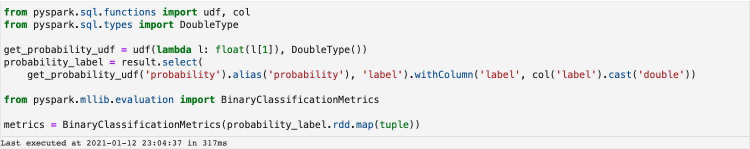
We will use log loss and Area under the ROC curve or AUC to evaluate the quality of model. Log loss is a standard evaluation criterion for events such as click-through rate prediction. The ROC curve shows the ratio of false positive rate (FPR) and true positive rate (TPR) when we liberalize the threshold to give a positive prediction.

In this tutorial, because CTR prediction is a binary classification problem, we use BinaryClassificationMetrics in Spark ML to compute metrics. We prepare a tuple <probability, label> for metrics computation.

ROC and AUC

A receiver operating characteristic curve, or ROC curve, is a graph that shows the performance of a classification model at all classification thresholds. This curve plots two parameters: True Positive Rate (TPR) and False Positive Rate (FPR). A higher Area under the ROC curve or AUC means the model is better at differentiating the classes.

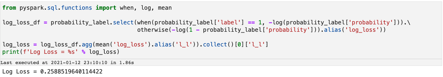
Log Loss

Log loss is the most important classification metric based on probabilities. For a given problem, a lower log loss value means better predictions.

CTR distribution

Feature engineering on 1B dataset

After our exploring on the small dataset, we go through the same feature engineering process on the 1B dataset and prepare data for model training. Our solution works well on data of this size.

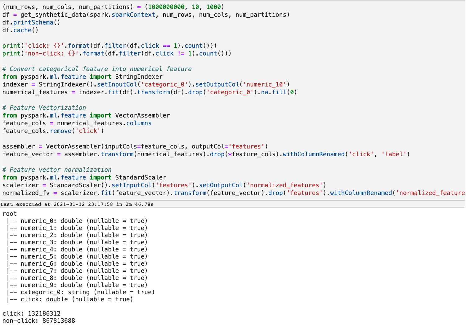
After completing the model training and evaluation on the 1B dataset, the AUC and log loss are as follows:

Multi-tenant

After you complete this tutorial, you can call the spark.stop() API. Spark will terminate itself in seconds, and the compute resources will be returned to the Amazon EKS cluster. Finally, when you’re done using Amazon EKS cluster, you should delete the resources associated with it so that you don’t incur any unnecessary costs. One of the major benefits of running workloads on Kubernetes is that the heterogeneous workloads (Spark, Services, Tooling etc.) and infrastructure tenants (users, projects etc.) can share the same compute environment. And resource-intensive jobs can use the idle resources when there aren’t many active jobs.

Conclusion

This blog post covered the problem of click prediction in digital advertising and a typical workflow of feature engineering and model training. Amazon EKS makes it possible to create Spark cluster in just a few minutes. It provides serverless experience so users no longer need to worry about hardware provisioning. It also offers a higher degree of resource sharing so that users can run larger scale jobs in a more cost-effective way.

You’ll find the code used in this blog post at https://github.com/aws-samples/eks-ctr-modeling-example-using-spark.