AWS Database Blog
Data preparation for machine learning using Amazon Timestream
Precognition, the ability to see events in the future, has always fascinated humankind. We probably will get there someday, but time series forecasting gets you close. The human brain is naturally trained to anticipate future events by analyzing the past, but the brain often makes only linear predictions because it can’t analyze the amount of data generated in a modern enterprise. How about letting a machine record those past sequences of events from millions of sources, analyze the data, and make predictions for your business?
Let’s take for example a software as a service (SaaS) provider that has thousands of customers from different industries, including online retail, oil and gas, and airline. The SaaS provider operates an infrastructure with Amazon Elastic Compute Cloud (Amazon EC2) instances running in multiple Regions and Availability Zones to provide low latency and highly available services to its customers. Both the service provider and its customers need detailed visibility into constantly changing operational activities. Aggregation of operational metrics for different time windows can give you visibility into the trends and patterns. You can then use this insight to adjust the infrastructure to adapt to the changing needs. You can also forecast the operational dynamics needed in the future to support optimal scale and therefore minimal costs, making the collected data actionable.
To store, transform, and analyze the operational data, the SaaS provider needs a database that can do the following:
- Persist trillions of data points per day in a cost-effective manner
- Support data preparation at the scale of petabytes for data science and machine learning (ML)
Although persistence of time series data can be custom implemented in any traditional databases, scale and usability is key here. For the SaaS provider with thousands of customers and tens of thousands of machines emitting time-based metrics and events, database scale and growth becomes a challenge. Amazon Timestream is a purpose-built time series database that allows you to collect and store millions of operational metrics per second and analyze that data in real time to improve application performance and availability.
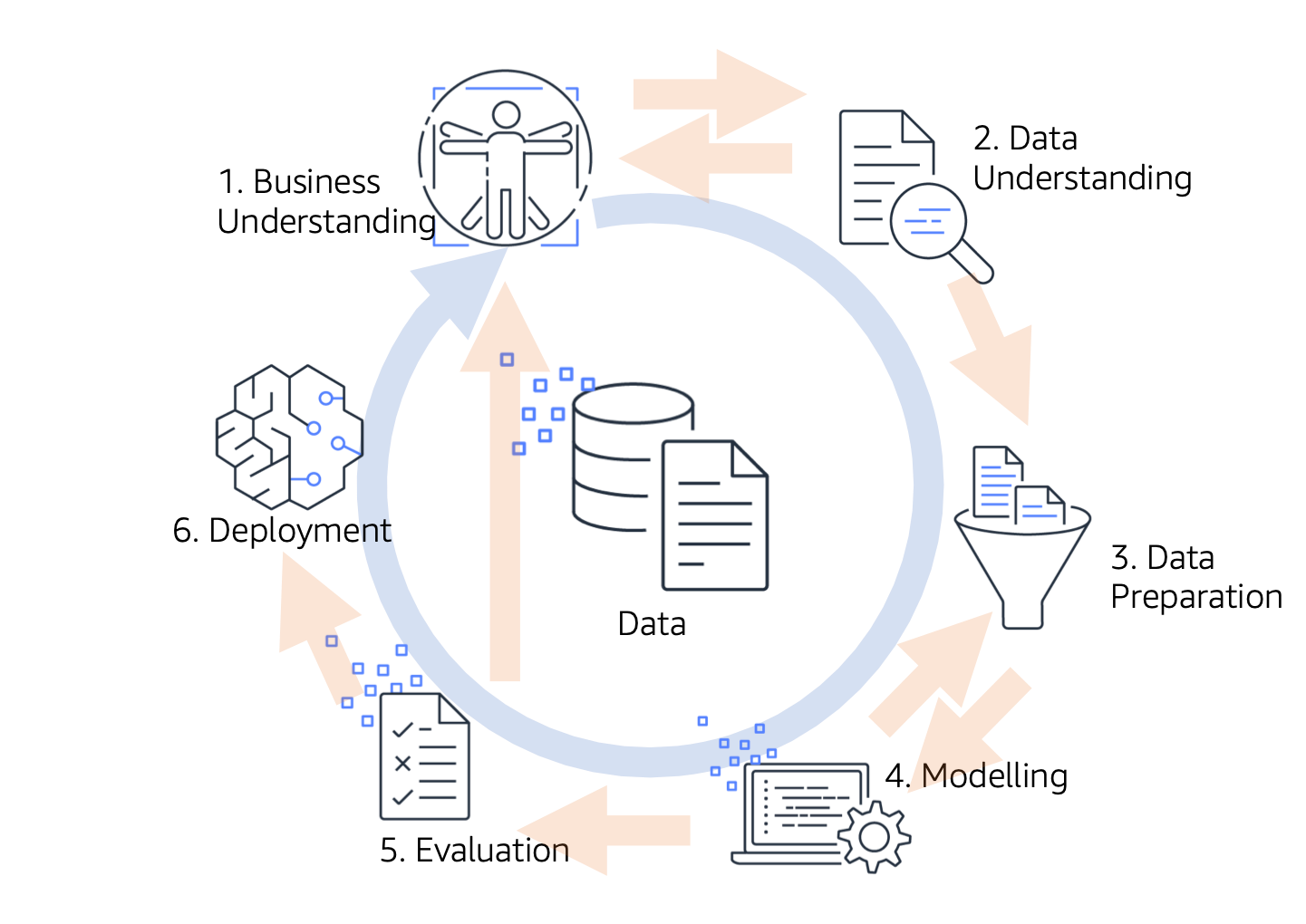
In this post, we describe how to use Timestream in the context of ML in relation to the open standard process model Cross Industry Standard Process for Data Mining (CRISP-DM). We focus specifically on the Data Understanding and Data Preparation phases, as shown in the following diagram, which are considered prerequisite to building highly accurate ML models. CRISP-DM defines generic tasks within these two phases as collect, describe, explore, and verify in the Data Understanding phase and select, clean, construct, integrate, and format data in the Data Preparation phase.
The powerful purpose-built query engine of Timestream, with its specialized time series functions, is designed for fast and efficient exploration and verification of the temporal data at hand. The Timestream SQL query engine allows many common data preparation operations so you can avoid the need for batch-based data preparation and preprocessing. You do this with queries in Timestream, which we explain later in this post.
The advantages of using Timestream query engine over the traditional method of batch loading and processing of data are as follows:
- Performance – Implementing data preparation within a query usually requires less computational work on the ML side, because the compute is closer to storage. Compare that to a two-step or multi-step extract, transform, and load (ETL) approach. The serverless architecture of Timestream supports fully decoupled data ingestion, storage, and query processing systems that can scale independently.
- Scalability and elasticity – In a traditional approach, scaling data preparation to millions of time series over very long periods requires self-managed horizontal and vertical scaling of infrastructure, with a huge amount of data required to be kept in an in-memory database to meet the performance needs. Timestream takes on that undifferentiated heavy lifting because it is serverless, and scales on demand to meet data scientists’ needs.
- Live application and sharing of queries – Query-based data preparation operates on the most recent data, whereas the result of a long-running ETL job might become stale. Sharing and keeping preprocessing scripts in sync across different technology stacks or even programming languages is very difficult. A Timestream query is reusable across all supported APIs and SDKs that are available in Java, Go, Python, Node.js, and .NET. Furthermore, you can share queries across phases and tools for visual data understanding in Amazon QuickSight and Grafana.
DevOps data generator
For this post, we extended the Timestream continuous ingestor tool from GitHub with a signal generator, which we can use to mix the random cpu_user signal with a periodic sinus or saw signal. You can then use the signal to noise ratio to define the ratio of signal strength to the uniformly distributed random values. For more details on the ingestion tool, see the README of the ingestor tool. Although the tool generates 20 different metrics from the DevOps domain, we focus on the cpu_user (CPU utilization between 0–100) and network_bytes_in/out (network traffic between 0 and 5 KB) metrics, and the time series of these measure values sharing the same dimensions (Region, cell, silo, Availability Zone, microservice name, and instance name).
To reproduce the simulated data and visualize it, you can run the following command for some minutes to generate and ingest sample data into Timestream:
The following figure has then been plotted using Amazon SageMaker Studio using the SageMaker notebook described in the Timestream and SageMaker integrations documentation. The following Python code shows how we queried Timestream and plotted the results:
The following plot shows our results.

Working with missing data
In this section, we focus on the required feature engineering task of dealing with time series missing data points. In a real-world DevOps scenario with thousands of servers emitting data, the missing data problem is common. Infrastructure scaling events (in or out), intermittent connectivity issues, and scheduled downtime are some of the reasons for missing data points. As we discussed before, in the Data Understanding phase, exploring the data and identifying such a problem is an important step before data preparation. To simulate the missing data problem, we used a data generator with the parameter —missing-cpu 25, which generates the cpu_user time series with 25% of the data points missing. One way to assess missing data occurrences is to plot the data and visually inspect it, which is easy for regular data but difficult in an irregular time series. We used the following query to retrieve
 cpu_user data from Timestream. A best practice is to limit the retrieved data to reduce the amount of data that needs to be scanned.
On the basis of the rawseries view, as defined in the preceding code, you can count the amount of time period assuming an equidistant time series and compare this with the number of values in a generated sequence for the same time period. If the actual and expected differ, one has missing values.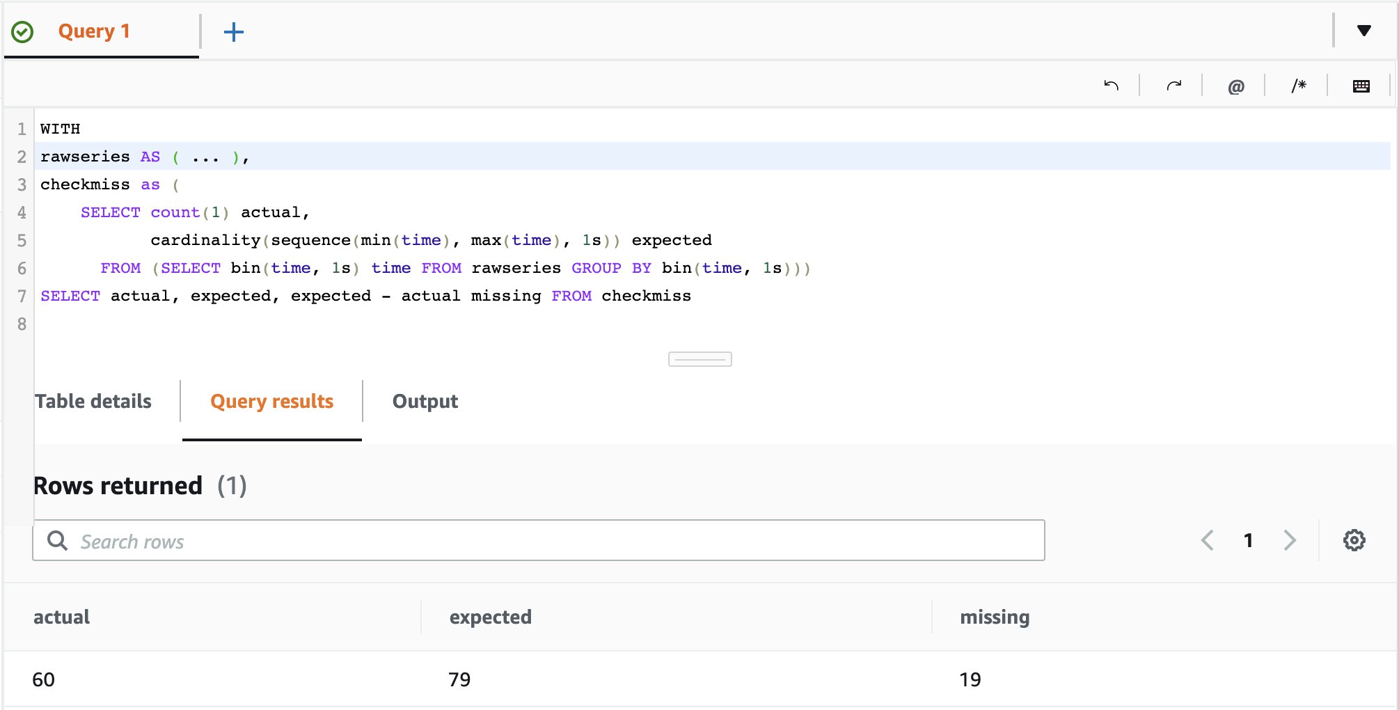 The query result showing 79 expected versus 60 existing values is the expected result from 25% missing data we ingested. Now that we have identified the issue, the next step is to fill these missing data gaps (Data Preparation). For this, we can use one of the interpolation functions in Timestream. For many use cases, a linear interpolation is a good fit; however, the last sampled value, cubic spline, and fixed values interpolation are also available for use (See Interpolation Functions for more details). The first and second figure in the following plot shows the time series as recorded and the result of the query using the
 interpolate_linear() function, where the gaps are now filled.
 For some algorithms, it works best to fill missing values with zeros, or any other fixed value. You can achieve this with the
 interpolate_fill() function:
The following plot shows our results.
We have just demonstrated how to use Timestream to prepare data with missing values for ML. The query-based approach is simple, easy to reuse, and can be applied to recent data, thereby avoiding the need to do batch processing.
Scaling features, normalization, and standardization
Scaling in data preparation is the technique of increasing or decreasing the relative size of time series values. Normalizing in data preparation is technique used to ensure that the data falls in a certain range. Scaling and normalization techniques can help reduce the numerical complexity, and improve the accuracy and runtime of algorithms. It also helps in better visualization of datasets with different ranges on the same plot. Most data scientists use min-max normalization, which ensures that all values of all time series fall between 0 and 1. In our DevOps example, the value ranges for cpu_user is between 0–100, but the values for network bytes I/O are in the range of 0–10,000.
The following formula shows how the min-max normalization is defined:

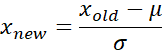
The following formula shows how z-Score standardization is defined:
Within Timestream, you can now create a query that calculates the min-max normalization on the fly and on the basis of the most recent data. This approach is also applicable for scenarios with sliding windows or unforeseen numerical changes in the data. See the following code:
The following plot shows within the first figure two signals being in a different numerical range, which leads to the aforementioned numerical complexity and makes visual analysis impossible. Applying the preceding min-max normalization to both signals projects the values to the interval [0..1], which is shown in the second plot.
Because outliers in the data might throw off normalization, another common approach to scale data in statistics and ML is the calculation of standard scores. This process ensures a mean value of zero and a variance of 1.
The following query, applied on both signals, projects the values as defined by the z-Score standardization:
The third plot illustrates these results. Large-scale data standardization
Although we show the preceding query-based standardization for a single time series, you can easily apply it for large-scale data preparation. As an example, we have ingested several billions of records using the continuous ingestor, simulating a microservice deployed in five Regions and on a total of 3,000 time series spread across Availability Zones, cells, silos, and instances. The query limited to a single time series returns with only 2.54 MB scanned in seconds with the standardized result:
We apply the same query for data preparation on all instances time series across the Availability Zones with the following code:
Due to the sorting, we can make sure that the first record is the same as the preceding query, but the query did scan in this case more than 6 GB of data and calculated the z-Score on 3,000 time series with more than 16.5 million measurements in seconds.
The rest of the queries in this use case are limited on single time series for simplicity of visualization and to keep the amount of data scanned low. However, as we detailed in this section, you can extend them to millions of time series because the Timestream query engine is built for processing the data at scale.
Dealing with trends and seasonality
Stationarity in a stochastic process means that statistical properties of the process don’t change over time. As a consequence, parameters such as mean and variance need to be stable over time. Because stationarity is often an underlying assumption in ML algorithms, transforming a non-stationary time series to stationary is an important data preparation step.
Naturally the operational dynamics in a SaaS scenario is non-stationary. If the business and customer base grow constantly, that leads to an underlying upwards trend in many of the metrics collected. Business applications also have a daily and weekly seasonality due to working hours and weekdays. With Timestream, you can craft queries that do the following:
- Help identify and quantify trends and seasonal effects
- Remove trends and seasonal effects to reach a stationary time series
The following figure on the left shows what a steady trend in a time series looks like, whereas the figure on the right shows clearly a seasonal trend. The time scale depends on the use case, but the approach to fix this with Timestream queries remains the same.
 |
 |
To make mean and variance stable over time, you can calculate the mean and variance over a sliding window and subtract the results from the raw time series, making the time series therefore piecewise stationary. You can achieve this by using the avg() aggregate function over a specific window in Timestream (see Window Functions and SQL Support). Such a query is shown in the following code block:
In this case, we calculate the linear trend as the mean of a large number of N historical values up to the current value. The calculated average has a temporal offset of N / 2 as shown in the following top figure, which can be dealt with by applying standardization as introduced earlier to the data. Using only historical data allows us to also use this preparation approach for time series prediction models. The second figure (bottom), shows the result of removing the linear trend from the recorded data and the derived new values. With the next query, we look into the second problem: a seasonal up/down as indicated by the second preceding figure. Depending on the ML task, it’s sometimes possible to take future data points into account, especially for anomaly detection problems, in which some future values are used as features. This approach with calculating the average on the preceding and following values in the OVER clause is shown in the following code block:
 Same as the preceding figures for the steady trend, the second figure shows the calculated new value with removed seasonal effects by simply subtracting the trend value of the recorded values. Note that in this case the average doesn’t have an offset because we used the preceding and following values.
In real-world problems, you can estimate these window parameters through external knowledge about the expected window size and verified visually or by calculating the root mean square error (RMSE). Timestream provides the query power, scale, and flexibility to integrate with tools like QuickSight, SageMaker, and Grafana to do so and experiment a lot.
In the preceding query, four preceding and four following measurements give a total window size of 9. Looping over different window sizes and visualizing them explains the brute force method used to derive these values for our given artificial data. As shown by the gray line graph in the following three figures, keeping the window size too small (window size = 3) shows more noise, resulting in removal of non-seasonal data that isn’t desired. On the other hand, keeping the window size too high (window size =35) flattens the trend too much, resulting in less than required reduction of seasonality.

Nearly all natural time series have some kind of seasonal bias, especially when human interaction are involved. Removing trends and ensuring stationarity of the time series often leads to better accuracy for ML algorithms like DeepAR+, CNN, and Random Cut Forrest (RCF).
To identify seasonal effects in time series, or repetitive underlying signals, analyzing the signal in the frequency domain is another way of identifying trends. A repeating signal shows, in the frequency domain, significant peaks at some frequencies. Because we’re dealing with discrete time series, we can use the Discrete Fourier Transformation (DTF) function from Timestream to derive the coefficients. Because the DTF can only be calculated on signals with equidistant sampling points not allowing for missing values, it might be necessary to apply the aforementioned technique of filling missing values. The result of DTF, the coefficient double array, represents the magnitude for the individual frequency bins in the frequency domain.
In the next figure, we plotted the noisy cpu_user signal from earlier, which has a seasonal trend of one sinus wave per minute (0.01667 Hz). The second plot (bottom) shows the signal in the frequency domain, as a result of the preceding DTF query. In the frequency domain, we clearly see expected spikes at 0Hz (the signal has a constant offset) and another peak at 0.01667 Hz (the season signal frequency); other frequencies are very low and can be seen as noise.
Although we have shown the advantages of Timestream when it comes to using queries for data insight and data preparation for the ML process from a qualitative perspective, we want to highlight here that you can apply these techniques to trillions of records and millions of time series data.
Conclusion
In this post, we demonstrated how to use the built-in functions in Timestream for data preparation and processing steps for ML. The high performant query engine of Timestream removes the undifferentiated heavy lifting of exporting the data, and performs custom development to apply feature engineering techniques. We showcased three commonly required feature engineering techniques for ML, using SQL-based Timestream query functions. Timestream allows you to query the database and therefore allows a higher reuse of queries. You can use Timestream for query-based data preparation at any scale, and it allows the database to be single source of truth, therefore you can share queries across different integration options.
To facilitate reproducing the queries reported in this post, we adapted the continuous ingestor tool, which is available on GitHub. Detailed instructions to use the generator can be found in the README. We also recommend following the best practices guide to optimize performance and query costs of your workload.
About the Authors
 Piyush Bothra is a Senior Solutions Architect with AWS where he helps customers innovate, differentiate their business, and transform their customer experiences. He has over 15 years’ experience helping customers achieve their business outcomes with architecture leadership and digital transformation enablement. Outside of work, Piyush loves spending time with family and friends, music, playing golf, and watching any live sports event.
 Andreas Juffinger is a Senior Solutions Architect with Amazon Web Services. He supports enterprise customers in building data intelligence platforms, lake house architectures and cloud native solutions solving technical and business challenges in strategic transformation programs. He has more than 20 years experience in data analytics, business intelligence and machine learning and a long history as lead application and enterprise architect.