AWS for SAP
Implementing a continual learning machine learning pipeline with Amazon SageMaker, AWS Glue DataBrew and SAP S/4HANA
Machine learning is increasingly becoming a core part of the digital transformation. It helps companies recognize patterns at scale and find novel ways to delight customers, streamline operations, or help make a product successful in a competitive marketplace. In practice, when you build an architecture based on machine learning, you need to understand the data, overcome the challenges involved in getting the data set right, and keep your model accurate with continuous feedback loop. In this blog post, we describe how to build end-to-end integration between SAP S/4HANA systems and Amazon SageMaker with a fast feedback loop leveraging the virtually unlimited capacity on AWS.
Introduction
We start off with the extraction SAP Data from a SAP S/4HANA systems using a combination of SAP OData, ABAP CDS and AWS Glue to move the data from SAP to an Amazon S3 bucket. We then use AWS Glue Databrew for data preparation and then using Amazon SageMaker for training the model. Finally, our prediction result is feedback to the SAP system.

Prerequisites
1. As an example, we are using credit card transaction data to simulate data within an SAP system. This can be downloaded from Kaggle.
2. Deployment of SAP S/4HANA. The easiest way to deploy this is using AWS LaunchWizard for SAP
Walk through
Step 1: SAP Data Preparations
There are number of ways to extract data from a SAP systems into AWS, here we are using ABAP Core Data Services (CDS) view, REST-based Open Data Protocol services (OData) and AWS Glue.
- In the SAP S/4HANA system, create a custom database table using SAP transaction
SE11. - Load the data from Kaggle into the SAP HANA table. The data from Kaggle is in CSV format and can be imported in the SAP HANA using the
IMPORT FROM CSVstatement. - Create SAP ABAP CDS view in the ABAP Development Tools (ADT). You can simply add the annotation
@OData.publish: trueto create an OData service. An example of this is available in the AWS Sample Github. - Activate OData service in SAP transaction
/IWFND/MAINT_SERVICE - Test the OData service in the SAP gateway client in SAP transaction
/IWFND/GW_CLIENT(Optional). - In the AWS Console, create an AWS Glue job for data extraction by following the AWS documentation for creating a Python shell job. You can find an example of the Python script in the AWS Sample Github. For our scenario, this took less than 1 minute to extract 284,807 entries from SAP using only 0.0625 Data Processing Unit (DPU).
Step 2: AWS Glue DataBrew for data wrangling
Before we start training the fraud detection modelling, we need to prepare the datasets to be ready for the machine learning training. Typically, this involves many steps like data cleansing, normalization, encoding and sometimes engineering new data features. AWS Glue DataBrew is a visual data preparation tool released in November 2020. This makes it easy for data analysts and data scientists to clean and normalize data up to 80% faster. You can choose from over 250 pre-built transformations to automate data preparation tasks, all without the need to write any code. In this section, we will walk you thought how easy it is to set this up.
Step 2.1 Create a Project
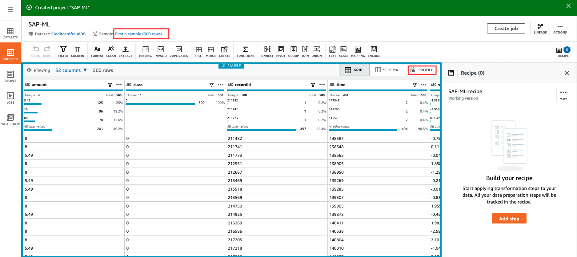
- Login to the AWS console and from top left corner choose service then AWS Glue DataBrew and select Create project.
- On the navigation pane, choose Projects, and then choose Create project.
- On the Project details pane, enter SAP-ML for the Project name.
- On the Select a dataset pane, choose New dataset.
- For Dataset name, enter
CreditcardfraudDB. - Here, we select Amazon S3 as the data source created in Step 1 and select Select the entire folder.
- For Access permissions, choose Create New IAM role and in suffix enter something like
fraud-detection-role. This is a service-linked role that allows DataBrew to read from your Amazon S3 input location. - Select Create Project

- AWS Glue DataBrew initially shows you a sample data set of 500 rows, but you can change this to include up to 5000 rows. This can either be the first, last or random rows.
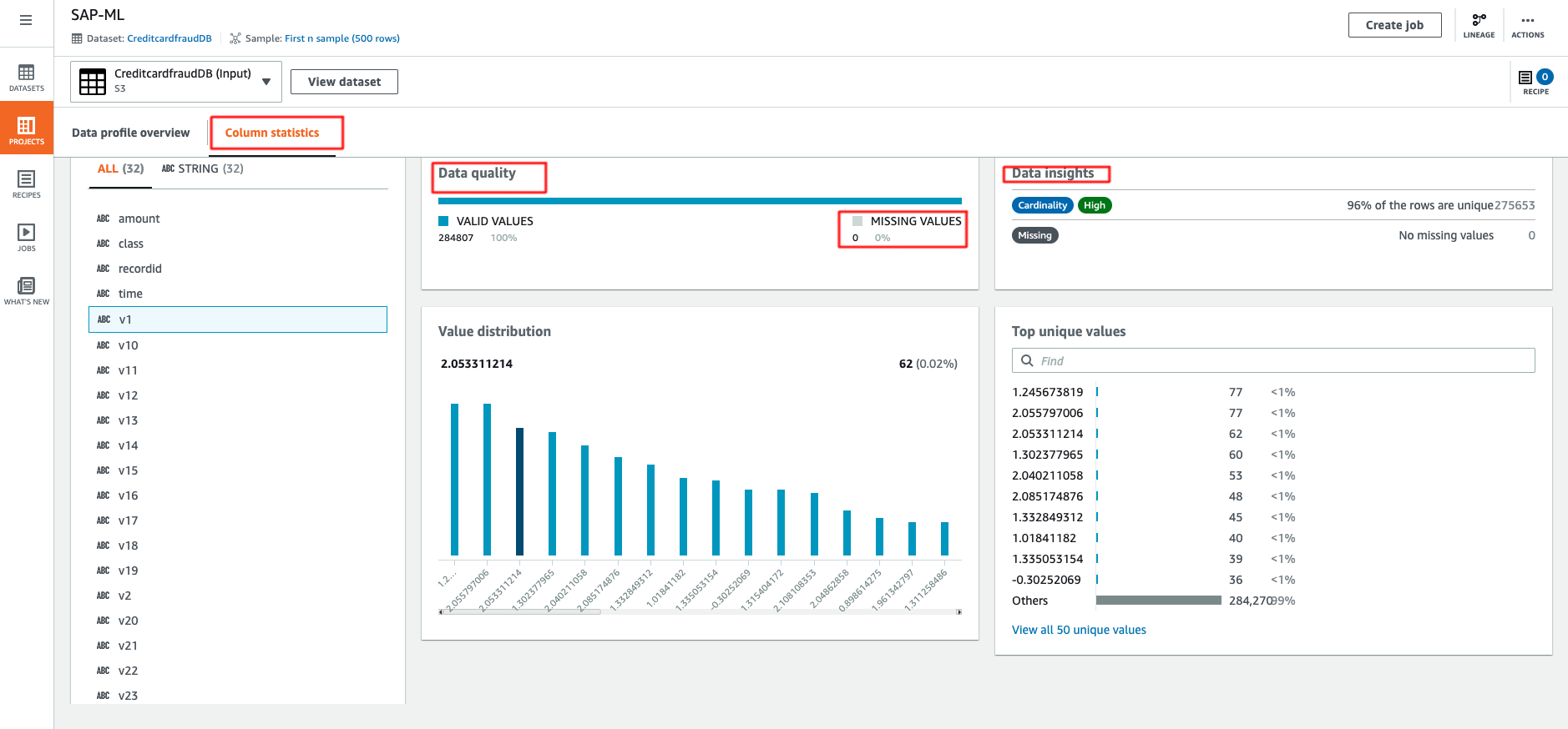
Step 2.2 Create Data Profile
One feature to highlight is that you can create a data profile to evaluate the quality of your datasets to understand data patterns and detect anomalies. This is very easy to use and you can follow the AWS documentation and and example output is shown below. By default, the data profile is limited to the first 20,000 rows of a dataset. However you can request a service limit increase for larger datasets. In our case, we requested an increase of the limit to 300,000 rows.
Glue DataBrew provides you with deeper insight about your dataset. Let’s deep dive into this. There are a total of 284,807 rows with 32 columns. There is no missing value, which is great news. Correlations is empty as the dataset has wrong schema, let’s take a look how easy it is to fix this.
Step 2.3 Data preparation
- The first step is to change data type for all columns. Select Schema and under Data type, change the type from
stringtonumber. AWS Glue DataBrew immediately calculate data statistics and generate a box plot for every single column once you changed the data type.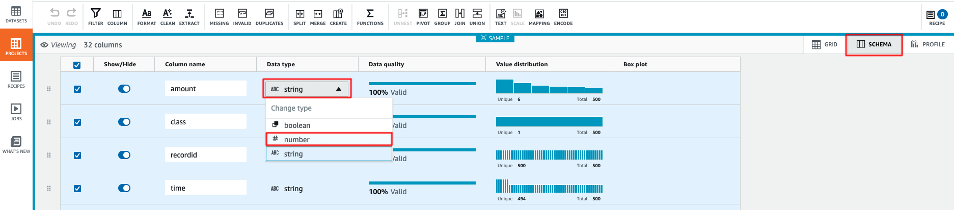
- Some machine learning algorithms are highly sensitive to feature scaling. This can cause algorithm to give a higher weighting for large values, and vice versa. In our data set, we use Z-score normalization to transform amount and time columns in the data to a same range and handle the outliers. Select Column Actions, then select Z-score normalization or standardization and select Apply. This creates 2 new columns called
amount_normalizedandtime_normalized. - In Column Action, Remove redundant columns by selecting
amount,timeandrecorded.Select Delete.
- Move the
classcolumn to the last. Select Column Action, then choose Move Column and End of the table. - Now we done with the required data transformation steps and we are ready to apply the configured transformation to the whole dataset. Select Create Job, enter the Job name
fraud-detection-transformationand choose the s3 folder destination for the output with file type CSV. - Alternatively, you can use a recipe to carry out the required transformation. You can find an example of this in the AWS Sample Github. Please refer to the AWS documentation on how to create recipe.
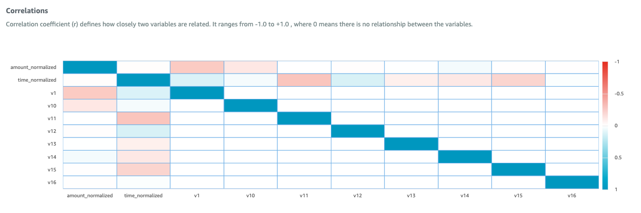
- As an optional step, you can import transformed data to AWS Glue DataBrew in a new project to validate the transformation and view features correlation matrix. The output is shown below.
Step 3: Amazon SageMaker
When you build an Machine Learning (ML)-based workload in AWS, you can choose from different levels of abstraction to balance speed to market with level of customization and ML skill level: ML Services, ML Frameworks and Infrastructure. In this blog post, we are using Amazon SageMaker. Amazon SageMaker is a fully-managed platform that enables developers and data scientists to quickly and easily build, train, and deploy machine learning. For this part of the solution, we are using Amazon SageMaker Studio.
- Follow the AWS documentation to launch the Amazon SageMaker Studio
- Clone the Jupyter note in AWS Sample Github.
- Select on
SAP_Fraud_Detection/SAP Credit Card Fraud Prediction.ipynband follow all instruction in the notebook carefully. Once you have completed all the steps in the Jupyter notebook successfully , the output is save in S3 bucket.
Step 4: SAP Data Import
Just like the data export in part 1, we are using ABAP CDS View, OData and AWS Glue. The steps here to create entry is different because the annotation @OData.publish: true does not support the CREATE ENTITY or CREATE ENTITY SET.
- In your SAP S/4HANA system, create a custom Z table using SAP transaction
SE11. - Create an SAP ABAP CDS view in the ABAP development tools (ADT).
- Create an OData services using SAP transaction
SEGWand then modify the code for the methodsCREATE ENTITYorCREATE ENTITY SET. You can find an example of this in the AWS Sample Github for this blog. - Activate your OData in SAP transaction
/IWFND/MAINT_SERVICE - In the AWS Console, create the AWS Glue job, an example code can be found in the AWS Sample Github.
Cleaning up
Cleaning up the infrastructure is easy, follow Amazon SageMaker clean up guide and AWS Glue DataBrew clean up guide to avoid incurring unnecessary charges. Also don’t forget about your S/4HANA system, and the data in Amazon S3, which needs to be deleted separately.
Conclusion
The value of data is dependent on your ability to interpret and model it quickly, and this capability is crucial in sustaining your competitive advantage. In this blog post, we show how to build a continuous machine learning pipeline using SAP data as the data sources. In particular, we focused on AWS Glue DataBrew and Amazon SageMaker to show you how this can help you speed up the process of getting faster feedback from the real world.
One important point is that building and using a machine learning model is not a one-way trip. The return trip that feeds the prediction result back to model building is just as important. Once you have successfully created a machine learning model with sufficient accuracy, it is likely that your model will need adjustment when there are new data or new business scenario. In order to maintain and continue to improve its accuracy, it is crucial to create a flywheel for machine learning.
If you have questions or would like to know about SAP on AWS innovations, please contact the SAP on AWS team using this link or visit aws.com/sap and aws.com/ml to learn more. Start building on AWS today and have fun!