AWS for SAP
Analytics at scale with Amazon Redshift lake house architecture using data from SAP and Amazon Connect
As a first step to business transformations, SAP on AWS customers relish the flexibility, agility, and scalability of the Amazon Web Services (AWS) platform and its support for the complete set of certified SAP offerings to run their business-critical SAP workloads. For some of our customers like Madrileña Red de Gas (MRG), the most immediate benefit has been the flexibility gained in the AWS Cloud, resulting in lower SAP infrastructure costs. But what inspires them the most is the broad range of technologies that AWS offers in the areas of Big Data, Machine Learning, Serverless Architecture and the omni-channel cloud based Amazon Connect Contact Center. With Amazon Connect Contact Center, they are lowering the barrier to innovation and running a cost-effective call center tool that continually improves their day to day operations. For more details, see the MRG case study.
As evolving cloud capabilities are transforming systems and IT landscapes for many companies, setting up a solid data and analytics platform to break their data silos typically takes precedence in their business transformation. As part of their transformation journey, customers need to collect data from various sources within the organization to create complex reporting capabilities that can provide a “single version of the truth” about various business events to make informed decisions and innovate. See building data lakes with SAP on AWS blog to learn about various data extraction patterns from SAP sources supported by SAP applications and third-party solutions.
In this blog, we will show how to set up a data and analytics platform to consolidate SAP data along with non-SAP application data to get better insights into the frequency of customer service calls. We will see how to use SAP Data Services – an application-level extractor – to extract the sales order data from SAP to Amazon Redshift for data warehousing, analyze the frequency of customer service calls with Amazon Connect data sets stored in Amazon Simple Storage Service (Amazon S3), and to use AWS Glue to transform the service call data and load the data to Amazon Redshift. For the reporting layer, we will use Amazon QuickSight and SAP Analytics Cloud to filter the frequency of customer service by sales order type.
Centralized lake house architecture using Amazon Redshift

Figure 1: Data extraction to Amazon Redshift using SAP Data services
For this blog, we will use SAP Operational Data Provisioning (ODP), a framework that enables data replication capabilities between SAP applications and SAP and non-SAP data targets using a provider and subscriber model. Let us start with the SAP source, and look at the steps involved.
Note: To create SAP data for demonstration and testing purposes. See the SAP NetWeaver Enterprise Procurement Model (EPM) documentation.
Prerequisites
For this tutorial, you should have the following prerequisites:
- An AWS account with the necessary permissions to configure Amazon Redshift, Amazon S3, AWS Glue and Amazon QuickSight.
- Ability to create source data in either SAP ECC or SAP S/4 HANA systems.
- Necessary permissions in SAP Data Services to configure data integration and transformation.
- Download the sample Contact Trace Records (CTR) JSON data model from Amazon S3 for post processing analytics exercise.
Creating an SAP Extractor
- Login to SAP transaction RSO2 in SAP and create a generic data-source for your SAP sales order tables.
- Enter desired name for your extractor (ex: ZSEPM_SALES) and click Create.
- In the next screen, select New_Hier_Root as application component and update the description fields with the desired texts.
- Enter the table SEPM_SDDL_SO_JOI as the data-source in the view/table field to extract the Sales order header and item details.
- Click “Generic Delta” in the menu choose “CHANGED_AT” as the field to filter changed records. You do this to extract delta or changed records after the initial load and Click Save.
- Validate your data-source using Data-Source Test Extraction option from the menu.
Creating Source Datastore in SAP Data Services
- Create a new project by choosing New from the SAP Data Services Designer Application menu and provide a desired name for your project.
- From the Data Services object library, create a new data-store with a desired name for Source DataStore and Datastore Type as SAP Applications from the drop down menu.
- Enter your SAP application server name, login credentials and update the SAP client in the advanced tab and click OK.
- Right-click on import by name from your new data-store ODP objects to import the data-source “ZSEPM_SALES” you created in SAP.
- Click next and assign the project name to the project created in step one.
- Choose “Changed-data capture (CDC) option and leave the field name blank and Click Import to import the SAP ODP object to the data-store.
You can use the SAP Landscape Transformation (SLT) Replication Server based Extractor as your Source data-store. See SAP Data Services and SAP LT Server for near real-time replication blog to configure SLT based data-source.
Creating the Redshift tables
- Create the Redshift target table in Redshift using the Redshift Query Editor or an SQL Client using the below DDL scripts. See Amazon Redshift documentation for steps to create Amazon Redshift Cluster.
CREATE TABLE SALESRS.SALESORDER (
MANDT	CHAR(3),
SALES_ORDER_KEY	VARCHAR(32),
SALES_ORDER_ID	CHAR(10),
TOTAL_GROSS_AMOUNT	DECIMAL(18,2),
TOTAL_NET_AMOUNT	DECIMAL(18,2),
TOTAL_TAX_AMOUNT	DECIMAL(18,2),
CREATED_BY_EMPLOYEE_ID	CHAR(10),
CHANGED_BY_EMPLOYEE_ID	CHAR(10),
CREATED_BY_BUYER_ID	CHAR(10),
CHANGED_BY_BUYER_ID	CHAR(10),
IS_CREATED_BY_BUYER	CHAR(1),
IS_CHANGED_BY_BUYER	CHAR(1),
CREATED_BY_ID	CHAR(10),
CHANGED_BY_ID	CHAR(10),
CREATED_AT	DECIMAL(21,7),
CHANGED_AT	DECIMAL(21,7),
HEADER_CURRENCY_CODE	CHAR(5),
DELIVERY_STATUS	CHAR(1),
LIFECYCLE_STATUS	CHAR(1),
BILLING_STATUS	CHAR(1),
BUYER_ID	CHAR(10),
BUYER_NAME	CHAR(80),
HEADER_ORIGINAL_NOTE_LANGUAGE	CHAR(1),
HEADER_NOTE_LANGUAGE	CHAR(1),
HEADER_NOTE_TEXT	CHAR(255),
ITEM_POSITION	CHAR(10),
ITEM_GROSS_AMOUNT	DECIMAL(18,2),
ITEM_NET_AMOUNT	DECIMAL(18,2),
ITEM_TAX_AMOUNT	DECIMAL(18,2),
ITEM_CURRENCY_CODE	CHAR(5),
ITEM_ORIGINAL_NOTE_LANGUAGE	CHAR(1),
ITEM_NOTE_LANGUAGE	CHAR(1),
ITEM_NOTE_TEXT	CHAR(255),
ITEM_PRODUCT_ID	CHAR(10),
ITEM_QUANTITY	DECIMAL(13,3),
ITEM_QUANTITY_UNIT	CHAR(3),
ITEM_DELIVERY_DATE	DECIMAL(21,7)
)
diststyle auto;
Creating the Target Datastore in SAP Data Services
- From the Data Services object library, create a new data-store with a desired name for Target DataStore and choose Datastore Type as “Amazon Redshift”.
- Click the ODBC connection setup for the connection to your Redshift cluster.
- From your DataSource name, click the ODBC Admin feature and click the configure option under the System DSN.
- Enter the Amazon Redshift Server, Port, Database name and user credentials for Auth type standard. Validate the connection by clicking Test. Then Click OK.
- Choose the new DataSource Name you created for your target Datastore and Click OK.
- From your new datastore, right click to choose “Import By Name” option to import the Amazon Redshift database table definition.
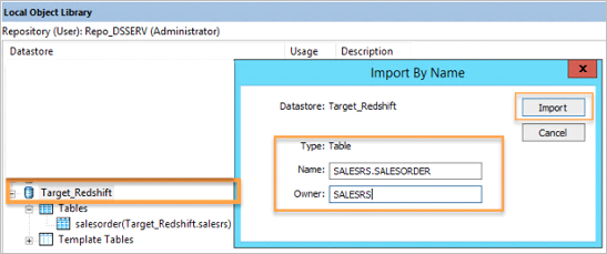
Figure 2: Importing target database tables
Creating data flow in SAP Data services
- From the SAP Data Services Project Area, right click to create “New Batch Job” with desired job name.
- Click on the new job created and drag the data flow option from the SAP Data Service Palette to create new data flow with desired data flow name.

Figure 3: Create Data Flow
Configure work flow in SAP Data services
- Click on the data flow created in the previous step, to access the data flow work space.
- Create a workflow by dragging and dropping the source ODP datasource (example: ZSEPM_SALES) from the datastore.
- Drag the query object from the transforms tab to the data flow workspace and connect it to the ODP object.
- Drag the query object the target Redshift SalesOrder datastore tables to the data flow workspace and connect the objects.
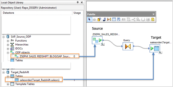
Figure 4: Source and Target Data flow setup
Ingest data to Amazon Redshift
- Double click the source datastore in the workflow, set the “Initial load” to Yes for the initial load.
- Click on the Query Transformation, and map the source fields to the target fields by “Map to Output” option.
- Now you can execute the Sales Order job to ingest the data to Amazon Redshift, and you can check the data that is loaded in the target Redshift database.
Optional Transformation
You can transform the data on the way to the target using the query transformation. Here we will add a regular expression to remove any special characters in the dataset before ingesting to Amazon Redshift Target. e.g To remove special characters in HEADER_NOTE_TEXT you can use a regular expression function regex_replace(<input_string/column_name>, ‘\[^a-z0-9\]’, ”, ‘CASE_INSENSITIVE’)
To add a transformation, choose the Query transformation, and ‘item_note_text’ in the Schema Out section. Under Mapping tab add the below regular expression function
regex_replace(ZSEPM_SALESORDER_S4HANATOREDSHIFT.HEADER_NOTE_TEXT, '\[^a-z0-9\]', '', 'CASE_INSENSITIVE')

Figure 5: Removing special characters from Header_Text
Change Data Capture with SAP Data Services (CDC)
Both Source and Target Based CDC are supported by SAP Data Services for databases. See SAP documentation to learn about CDC options.
Note: SAP Data Services also supports SAP database level extraction from SAP as a source to access the underlying SAP tables. See SAP documentation to configure native ODBC data sources.
Amazon Connect setup to stream data to Amazon Redshift
Amazon Connect can be integrated with Amazon Kinesis to stream Contact Trace Records (CTRs) into Amazon Redshift. See Amazon Connect QuickStart documentation on setting up and integrating Amazon Connect data. Also, see Amazon Connect administration guide to review the Contact Trace Records (CTR) data model. You can ingest the contact trace records into Amazon Redshift, and join this data with the Sales Order details that you replicated from SAP source systems.
You can add any key value pairs to a CTR using contact attributes in the contact flow. You can add the SalesOrderId as a key value pair into a CTR using contact attribute “SAPOrder”. See, Amazon Connect administration guide for information on how to use contact attributes to personalize the customer experience. For this example, we will use SalesOrderID to link the data in Amazon Connect to the Sales orders from SAP.
CTR JSON Data
For this post, we will use the JSON data that is already created with a custom attribute and available in S3 location here. This is a JSON dataset from Amazon Connect workflow with a custom attribute “SAPOrder” added for the Agent to enter the OrderId related to the enquiry.
You can use this data to link the SAP orders extracted from SAP source system to analyze the order inquiries.This is a JSON dataset from Amazon Connect workflow with a custom attribute “SAPOrder” added for the Agent to enter the OrderId related to the enquiry. You can use this data to link the SAP orders extracted from SAP source system to analyze the order inquiries.
Creating Glue catalog by crawling the CTR data
- Upload the sample CTR JSON file to Amazon S3 bucket in your Amazon account.
- Open AWS Glue in AWS console, and create a new crawler by choosing “Crawler” and “Add Crawler”

Figure 6: Adding AWS Glue Crawler
Adding data store in AWS Glue
- You can use desired name for your crawler, for this example we will use amazonconnectsaplink as crawler name and choose Next in the next two screens.
- In Add a data store screen, enter or choose the Amazon S3 bucket name where you uploaded the Amazon Connect CTR file and choose Next.

Figure 7: Specify the Source S3 Bucket path
Executing AWS Crawler
- Select no for Add another data store, and choose Next.
- Select Create an IAM role, AWSGlueServiceRole-ConnectSAP, and enter a name for the IAM role and choose Next.
- Select Run on demand for Frequency and choose Next.
- Choose Add database option and enter a desired database name under which you want to create the Glue catalog tables. For this example, we will enter amazonconnect.
- Click Finish.
- You should see the new crawler you just created. Select the Crawler and click Run crawler option.
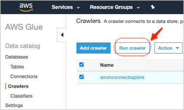
Figure 8: Executing Glue Crawler
After the crawler completes running, you should see the table amznconnectsapordlink in your Glue Database.
Data modeling in Amazon Redshift
Amazon Redshift is a columnar store, massively parallel processing (MPP) data warehouse service, which provides integration to your data lake to enable you to build highly scalable analytics solutions.
Similar to calculation views in SAP HANA, you can create Amazon Redshift database views to build business logic combining tables. Redshift extends this capability to materialized views, where you can store the pre-computed results of queries and efficiently maintain them by incrementally processing the latest changes made to the source tables. Queries executed on the materialized views use the pre-computed results to run much faster.
- Create a new Amazon Redshift cluster. See Amazon Redshift documentation for steps to create a cluster.
- Ensure that your AWS IAM roles attached to Redshift cluster has necessary read and write IAM policies to access AmazonS3, AWS Glue. Note: AmazonS3 should allow export of data from Amazon Redshift to Amazon S3. AWSGlueConsoleFullAccess is required to create a Glue catalog and enable query of CTR data using Amazon Redshift Spectrum.
- Login to Amazon Redshift using query editor. You can also use a SQL Client Tool ike DBeaver in this case. See, Amazon Redshift documentation to configure connection between SQL client tools and Amazon Redshift.
- Execute the external schema statement from the below code snippet. Alter the code snippet to use the appropriate AWS Glue data catalog database and the IAM role ARN you created in previous steps.
- Validate the new external schema and the external table in your Amazon Redshift database which should point to the Amazon Connect CTR data in S3.
drop schema if exists amazonconnect_ext;
create external schema amazonconnect_ext
from data catalog database 'amazonconnect'
iam_role 'arn:aws:iam:: <AWSAccount>:role/mySpectrumRole';
Consolidating data for unified view
- Execute the query from the below code snippets to combine the SAP Sales order data loaded from Data services and Amazon Connect CTR data in S3 and add transformations for call initiationtimestamp and add dimensions week, month, year, dayofmonth to enable ad-hoc analysis.
create table sapsales.amznconnectsaporder
as select amzcsap.awsaccountid, amzcsap.saporder , amzcsap.agent.AgentInteractionDuration as aidur,
   amzcsap.awscontacttracerecordformatversion, amzcsap.channel, amzcsap.queue.arn as arn,
	TO_TIMESTAMP(amzcsap.connectedtosystemtimestamp,'YYYY-MM-DD HH24:MI:SS')  callconnectedtosystemtimestamp,
   	TO_TIMESTAMP(amzcsap.initiationtimestamp,'YYYY-MM-DD HH24:MI:SS') callinitiationtimestamp,
   	TO_DATE(amzcsap.initiationtimestamp,'YYYY-MM-DD') callinitiationdate,
	date_part(w, to_date(amzcsap.initiationtimestamp,'YYYY-MM-DD')) as callinitweek,
	date_part(mon, to_date(amzcsap.initiationtimestamp,'YYYY-MM-DD')) as callinitmonth,
	date_part(dow, to_date(amzcsap.initiationtimestamp,'YYYY-MM-DD')) as callinitdow,
	date_part(yr, to_date(amzcsap.initiationtimestamp,'YYYY-MM-DD')) as callinityear,
	date_part(d, to_date(amzcsap.initiationtimestamp,'YYYY-MM-DD')) as callinitdom
from amazonconnect_ext.amznconnectsapordlink amzcsap;
Note: You can execute the query from the below code snippet to create a view with desired data for visualization. This query can also be created as a materialized view to improve performance of this view. See Amazon Redshift documentation to create materialized views in Amazon Redshift.
create view sapsales.v_orderenquiryanalytics
as select amzcsap.awsaccountid, amzcsap.saporder, amzcsap.aidur,
   amzcsap.awscontacttracerecordformatversion, callconnectedtosystemtimestamp, callinitiationtimestamp,callinitiationdate,
   amzcsap.channel, amzcsap.arn, sapord.sales_order_key, sapord.buyer_id, sapord.buyer_name,
	sapord.item_gross_amount, sapord.item_product_id, sapord.item_delivery_date, sapord.created_at,
	callinitweek,
	callinitmonth,
	callinitdow,
	callinityear,
	callinitdom
from sapsales.amznconnectsapord amzcsap, sapsales.salesorder sapord
where amzcsap.saporder = sapord.sales_order_id;
Validate the data output
Execute the query from the below code snippet to validate the data output for your analytics.
a. Top 10 buyers with most frequency and duration of calls
select buyer_id, buyer_name, sum(aidur) as callduration
from sapsales.v_orderenquiryanalytics
group by buyer_id, buyer_name
order by callduration desc
limit 10;
b. Products causing more connect calls
select item_product_id, sum(aidur) as callduration
from sapsales.v_orderenquiryanalytics
group by item_product_id
order by callduration desc
limit 10;
Visualization using Amazon QuickSight
- Login to Amazon QuickSight from the AWS Management Console.
- Choose Data Sets, and create a new data set.
- Enter a desired name for your data source.
- Chose the Amazon Redshift Instance ID, and enter the Database name, Username and Password.
- Choose Create Data Source.
- Choose the schema (example: sapsales) created in Amazon Redshift earlier.
- Choose the Redshift table (example: orderenquiryanalytics) you created in the previous step.
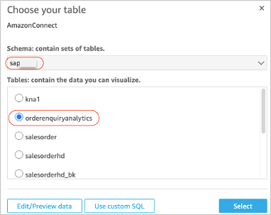
Figure 9: Choosing the Amazon Redshift Schema in Quicksight
Setting up the Visualization
- Choose Directly query your data and click Visualize.
- On the visualize screen, choose +Add and click Add visual on the top left of the screen multiple times to create 4 visuals.
- For the first visual type, choose Vertical bar chart. Choose the first visual select aidur for y-axis and buyer_name for x-axis from the fields list.
- For the second visual, choose Pie chart for visual type and visual select aidur, and month.
- For the third visual, choose Horizontal bar chart for visual type and select aidur for x-axis and item_product_id for y-axis.
- For the fourth visual, choose Scatter plot chart and select dow for x-axis and aidur for y-axis.
- Finally, you should see the visualization as shown below.

Figure 10: Amazon QuickSight Dashboard
Modeling using SAP HANA Studio
If you want to use HANA Studio or SAP Analytics Cloud as your modeling and front-end tool of choice, then you can connect to Amazon Redshift using Smart Data Access (SDA). Amazon Redshift view or materialized view can be accessed from SAP HANA Studio using the Simba connector. For more details on SDA, see SAP documentation on SAP HANA Smart Data Access .

Figure 11: Adding remote data source in SAP HANA
Visualize unified data using SAP Analytics Cloud
You can use the unload command to store the results your Redshift query as csv files to an Amazon S3 bucket for SAP Analytics Cloud (SAC) visualization. See Amazon Redshift documentation for unload examples.

Figure 12: SAP Analytics Cloud Visualization with Amazon S3 data.
Note: You can also use SAC reporting layer to connect to Amazon Redshift using APOS live data gateway.
Summary
Enterprises are increasingly turning to data lakes to track and optimize business performance. In this blog, we demonstrated how to establish a data lake that consolidates SAP and non-SAP data for deeper customer insight using SAP Data Services to extract data to Amazon Redshift for data warehousing to provide a unified view of data from both Amazon Connect and SAP.
To get started, visit aws.amazon.com/redshift. To learn more about running SAP on AWS, visit aws.amazon.com/sap.