AWS Big Data Blog
Migrate to an Amazon Redshift Lake House Architecture from Snowflake
The need to derive meaningful and timely insights increases proportionally with the amount of data being collected. Data warehouses play a key role in storing, transforming, and making data easily accessible to enable a wide range of use cases, such as data mining, business intelligence (BI) and reporting, and diagnostics, as well as predictive, prescriptive, and cognitive analysis.
Several new features of Amazon Redshift address a wide range of data requirements and improve performance of extract, load, and transform (ELT) jobs and queries. For example, concurrency scaling, the new RA3 instance types, elastic resize, materialized views, and federated query, which allows you to query data stored in your Amazon Aurora or Amazon Relational Database Service (Amazon RDS) Postgres operational databases directly from Amazon Redshift, and the SUPER data type, which can store semi-structured data or documents as values. The new distributed and hardware accelerated cache with AQUA (Advanced Query Accelerator) for Amazon Redshift delivers up to10 times more performance than other cloud warehouses. The machine learning (ML) based self-tuning capability to set sort and distribution keys for tables significantly improves query performance that was previously handled manually. For the latest feature releases for AWS services, see What’s New with AWS?
To take advantage of these capabilities and future innovation, you need to migrate from your current data warehouse, like Snowflake, to Amazon Redshift, which involves two primary steps:
- Migrate raw, transformed, and prepared data from Snowflake to Amazon Simple Storage Service (Amazon S3)
- Reconfigure data pipelines to move data from sources to Amazon Redshift and Amazon S3, which provide a unified, natively integrated storage layer of our Lake House Architecture
In this post, we show you how to migrate data from Snowflake to Amazon Redshift. We cover the second step, reconfiguring pipelines, in a later post.
Solution overview
Our solution is designed in two stages, as illustrated in the following architecture diagram.

The first part of our Lake House Architecture is to ingest data into the data lake. We use AWS Glue Studio with AWS Glue custom connectors to connect to the source Snowflake database and extract the tables we want and store them in Amazon S3. To accelerate extracting business insights, we load the frequently accessed data into an Amazon Redshift cluster. The infrequently accessed data is cataloged in the AWS Glue Data Catalog as external tables that can be easily accessed from our cluster.
For this post, we consider three tables: Customer, Lineitem, and Orders, from the open-source TCPH_SF10 dataset. An AWS Glue ETL job, created by AWS Glue Studio, moves the Customers and Orders tables from Snowflake into the Amazon Redshift cluster, and the Lineitem table is copied to Amazon S3 as an external table. A view is created in Amazon Redshift to combine internal and external datasets.
Prerequisites
Before we begin, complete the steps required to set up and deploy the solution:
- Create an AWS Secrets Manager secret with the credentials to connect to Snowflake: username, password, and warehouse details. For instructions, see Tutorial: Creating and retrieving a secret.
- Download the latest Snowflake JDBC JAR file and upload it to an S3 bucket. You will find this bucket referenced as SnowflakeConnectionbucket in the cloudformation step.
- Identify the tables in your Snowflake database that you want to migrate.
Create a Snowflake connector using AWS Glue Studio
To complete a successful connection, you should be familiar with the Snowflake ecosystem and the associated parameters for Snowflake database tables. These can be passed as job parameters during run time. The following screenshot from a Snowflake test account shows the parameter values used in the sample job.

The following screenshot shows the account credentials and database from Secrets Manager.

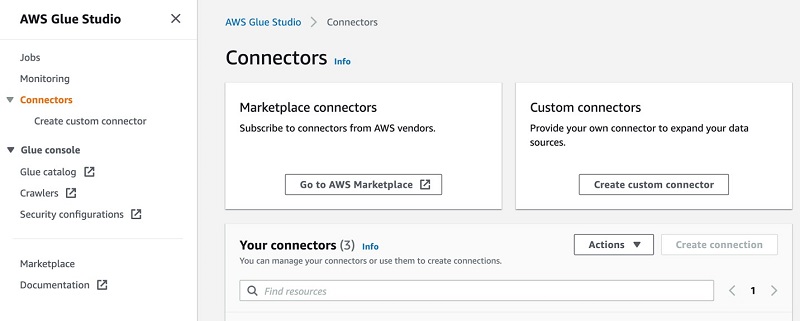
To create your AWS Glue custom connector for Snowflake, complete the following steps:
- On the AWS Glue Studio console, under Connectors, choose Create custom connector.
- For Connector S3 URL, browse to the S3 location where you uploaded the Snowflake JDBC connector JAR file.
- For Name, enter a logical name.
- For Connector type, choose JDBC.
- For Class name, enter
net.snowflake.client.jdbc.SnowflakeDriver. - Enter the JDBC URL base in the following format:
jdbc:snowflake://<snowflakeaccountinfo>/?user=${Username}&password=${Password}&warehouse=${warehouse}. - For URL parameter delimiter, enter &.
- Optionally, enter a description to identify your connector.
- Choose Create connector.

Set up a Snowflake JDBC connection
To create a JDBC connection to Snowflake, complete the following steps:
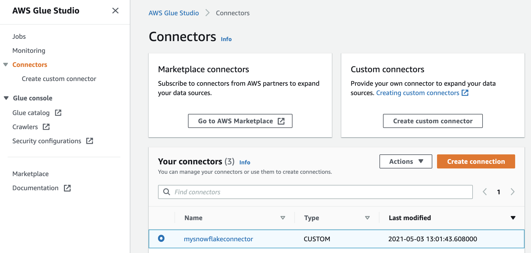
- On the AWS Glue Studio console, choose Connectors.
- Choose the connector you created.
- Choose Create connection.
- For Name and Description, enter a logical name and description for your reference.

- For Connection credential type, choose default.
- For AWS Secret, choose the secret created as a part of the prerequisites.
- Optionally, you can specify the credentials in plaintext format.
- Under Additional options, add the following key-value pairs:
- Key
dbwith the Snowflake database name - Key
schemawith the Snowflake database schema - Key
warehousewith the Snowflake warehouse name
- Key
- Choose Create connection.
Configure other resources and permissions using AWS CloudFormation
In this step, we create additional resources with AWS CloudFormation, which includes an Amazon Redshift cluster, AWS Identity and Access Management (IAM) roles with policies, S3 bucket, and AWS Glue jobs to copy tables from Snowflake to Amazon S3 and from Amazon S3 to Amazon Redshift.
- Sign in to the AWS Management Console as an IAM power user, preferably an admin user.
- Choose your Region as
us-east-1. - Choose Launch Stack:

- Choose Next.

- For Stack name, enter a name for the stack, for example,
snowflake-to-aws-blog. - For Secretname, enter the secret name created in the prerequisites.
- For SnowflakeConnectionName, enter the Snowflake JDBC connection you created.
- For Snowflake Connection bucket, enter name of the S3 bucket where the snowflake connector is uploaded
- For SnowflakeTableNames, enter the list of tables to migrate from Snowflake. For example,
Lineitem,customers,order. - For RedshiftTableNames, enter the list of the tables to load into your warehouse (Amazon Redshift). For example,
customers,order.

- You can specify your choice of Amazon Redshift node type, number of nodes, and Amazon Redshift username and password, or use the default values.
- For the MasterUserPassword, enter a password for your master user keeping in mind the following constraints : It must be 8 to 64 characters in length. It must contain at least one uppercase letter, one lowercase letter, and one number.
- Choose Create stack.
Run AWS Glue jobs for the data load
The stack takes about 7 minutes to complete. After the stack is deployed successfully, perform the following actions:
- On the AWS Glue Studio console, under Databases, choose Connections.
- Select the connection
redshiftconnectionfrom the list and choose Test Connection. - Choose the IAM role
ExecuteGlueSnowflakeJobRolefrom the drop-down meu and choose Test connection.

If you receive an error, verify or edit the username and password and try again.
- After the connection is tested successfully, on the AWS Glue Studio console, select the job
Snowflake-s3-load-job. - On the Action menu, choose Run job.


When the job is complete, all the tables mentioned in the SnowflakeTableNames parameter are loaded into your S3 bucket. The time it takes to complete this job varies depending on the number and size of the tables.
Now we load the identified tables in Amazon Redshift.
- Run the job
s3-redshift-load-job. - After the job is complete, navigate to the Amazon Redshift console.
- Use the query editor to connect to your cluster to verify that the tables specified in
RedshiftTableNamesare loaded successfully.
You can now view and query datasets from Amazon Redshift. The Lineitem dataset is on Amazon S3 and queried by Amazon Redshift Spectrum. The following screenshot shows how to create an Amazon Redshift external schema that allows you to query Amazon S3 data from Amazon Redshift.

Tables loaded to Amazon Redshift associated storage appear as in the following screenshot.

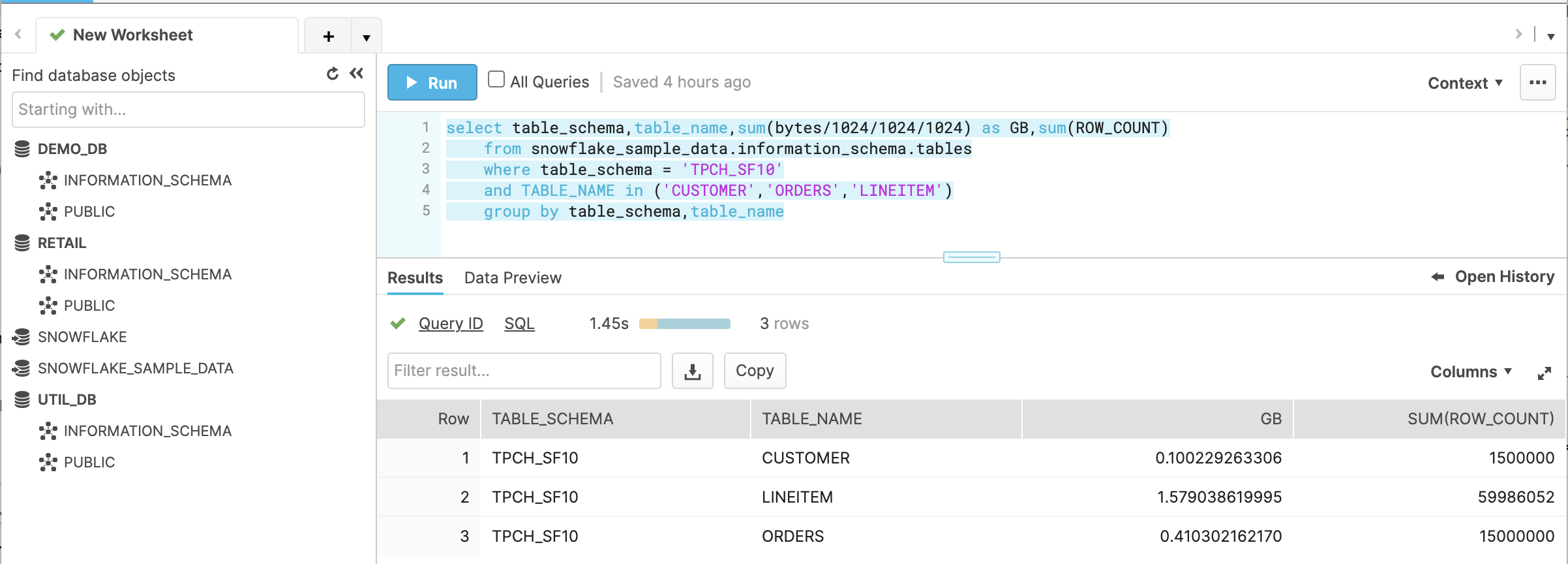
The AWS Glue job, using the standard worker type to move Snowflake data into Amazon S3, completed in approximately 21 minutes, loading overall 2.089 GB (about 76.5 million records). The following screenshot from the Snowflake console shows the tables and their sizes, which we copied to Amazon S3.
You have the ability to customize the AWS Glue worker type, worker nodes, and max concurrency to adjust distribution and workload.
AWS Glue allows parallel data reads from the data store by partitioning the data on a column. You must specify the partition column, the lower partition bound, the upper partition bound, and the number of partitions. This feature enables you use data parallelism and multiple Spark executors allocated the Spark application.
This completes our migration from Snowflake to Amazon Redshift that enables a Lake House Architecture and the ability to analyze data in more ways. We would like to take a step further and talk about features of Amazon Redshift that can help extend this architecture for data democratization and modernize your data warehouse.
Modernize your data warehouse
Amazon Redshift powers the Lake House Architecture, which enables queries from your data lake, data warehouse, and other stores. Amazon Redshift can access the data lake using Redshift Spectrum. Amazon Redshift automatically engages nodes from a separate fleet of Redshift Spectrum nodes. These nodes run queries directly against Amazon S3, run scans and aggregations, and return the data to the compute nodes for further processing.
AWS Lake Formation provides a governance solution for data stored in an Amazon S3-based data lake and offers a central permission model with fine-grained access controls at the column and row level. Lake Formation uses the AWS Glue Data Catalog as a central metadata repository and makes it simple to ingest and catalog data using blueprints and crawlers.
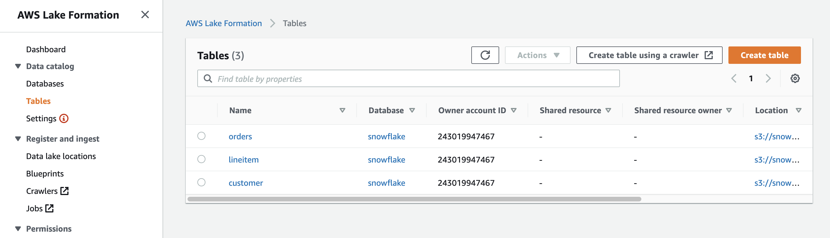
The following screenshot shows the tables from Snowflake represented in the AWS Glue Data Catalog and managed by Lake Formation.
With the Amazon Redshift data lake export feature, you can also save data back in Amazon S3 in open formats like Apache Parquet, to use with other analytics services like Amazon Athena and Amazon EMR.
Distributed storage
Amazon Redshift RA3 gives the flexibility to scale compute and storage independently. Amazon Redshift data is stored on Amazon Redshift managed storage backed by Amazon S3. Distribution of datasets between cluster storage and Amazon S3 allows you to benefit from bringing the appropriate compute to the data depending on your use case. You can query data from Amazon S3 without accessing Amazon Redshift.
Let’s look at an example with the star schema. We can save a fact table that we expect to grow rapidly in Amazon S3 with the schema saved in the Data Catalog, and dimension tables in cluster storage. You can use views with union data from both Amazon S3 and the attached Amazon Redshift managed storage.
Another model for data distribution can be based on the state of hot or cold data, with hot data in Amazon Redshift managed storage and cold data in Amazon S3. In this example, we have the datasets lineitem, customer, and orders. The customer and orders portfolio are infrequently updated datasets in comparison to lineitem. We can create an external table to read lineitem data from Amazon S3 and the schema from the Data Catalog database, and load customer and orders to Amazon Redshift tables. The following screenshot shows a join query between the datasets.

It would be interesting to know the overall run statistics for this query, which can be queried from system tables. The following code gets the stats from the preceding query using svl_s3query_summary:
The following screenshot shows query output.

For more information about this query, see Using the SVL_QUERY_SUMMARY view.
Automated table optimization
Distribution and sort keys are table properties that define how data is physically stored. These are managed by Amazon Redshift. Automatic table optimization continuously observes how queries interact with tables and uses ML to select the best sort and distribution keys to optimize performance for the cluster’s workload. To enhance performance, Amazon Redshift chooses the key and tables are altered automatically.
In the preceding scenario, the lineitem table had distkey (L_ORDERKEY), the customer table had distribution ALL, and orders had distkey (O_ORDERKEY).
Storage optimization
Choosing a data format depends on the data size (JSON, CSV, or Parquet). Redshift Spectrum currently supports Avro, CSV, Grok, Amazon Ion, JSON, ORC, Parquet, RCFile, RegexSerDe, Sequence, Text, and TSV data formats. When you choose your format, consider the overall data scanned and I/O efficiency, such as with a small dataset in CSV or JSON format versus the same dataset in columnar Parquet format. In this case, for smaller scans, Parquet consumes more compute capacity compared to CSV, and may eventually take around the same time as CSV. In most cases, Parquet is the optimal choice, but you need to consider other inputs like volume, cost, and latency.
SUPER data type
The SUPER data type offers native support for semi-structured data. It supports nested data formats such as JSON and Ion files. This allows you to ingest, store, and query nested data natively in Amazon Redshift. You can store JSON formatted data in SUPER columns.
You can query the SUPER data type through an easy-to-use SQL extension that is powered by the PartiQL. PartiQL is a SQL language that makes it easy to efficiently query data regardless of the format, whether the data is structured or semi-structured.
Pause and resume
Pause and resume lets you easily start and stop a cluster to save costs for intermittent workloads. This way, you can cost-effectively manage a cluster with infrequently accessed data.
You can apply pause and resume via the console, API, and user-defined schedules.
AQUA
AQUA for Amazon Redshift is a large high-speed cache architecture on top of Amazon S3 that can scale out to process data in parallel across many nodes. It flips the current paradigm of bringing the data to the compute—AQUA brings the compute to the storage layer so the data doesn’t have to move back and forth between the two, which enables Amazon Redshift to run queries much faster.
Data sharing
The data sharing feature seamlessly allows multiple Amazon Redshift clusters to query data located in RA3 clusters and their managed storage. This is ideal for workloads that are isolated from each other but data needs to be shared for cross-group collaboration without actually copying data.
Concurrency scaling
Amazon Redshift automatically adds transient clusters in seconds to serve sudden spikes in concurrent requests with consistently fast performance. For every 1 day of usage, 1 hour of concurrency scaling is available at no charge.
Conclusion
In this post, we discussed an approach to migrate a Snowflake data warehouse to a Lake House Architecture with a central data lake accessible through Amazon Redshift.
We covered how to use AWS Glue to move data from sources like Snowflake into your data lake, catalog it, and make it ready to analyze in a few simple steps. We also saw how to use Lake Formation to enable governance and fine-grained security in the data lake. Lastly, we discussed several new features of Amazon Redshift that make it easy to use, perform better, and scale to meet business demands.
About the Authors
 Soujanya Konka is a Solutions Architect and Analytics specialist at AWS, focused on helping customers build their ideas on cloud. Expertise in design and implementation of business information systems and Data warehousing solutions. Before joining AWS, Soujanya has had stints with companies such as HSBC, Cognizant.
 Shraddha Patel is a Solutions Architect and Big data and Analytics Specialist at AWS. She works with customers and partners to build scalable, highly available and secure solutions in the AWS cloud.