AWS Big Data Blog
Power enterprise-grade Data Vaults with Amazon Redshift – Part 1
Amazon Redshift is a popular cloud data warehouse, offering a fully managed cloud-based service that seamlessly integrates with an organization’s Amazon Simple Storage Service (Amazon S3) data lake, real-time streams, machine learning (ML) workflows, transactional workflows, and much more—all while providing up to 7.9x better price-performance than other cloud data warehouses.
As with all AWS services, Amazon Redshift is a customer-obsessed service that recognizes there isn’t a one-size-fits-all for customers when it comes to data models, which is why Amazon Redshift supports multiple data models such as Star Schemas, Snowflake Schemas and Data Vault. This post discusses best practices for designing enterprise-grade Data Vaults of varying scale using Amazon Redshift; the second post in this two-part series discusses the most pressing needs when designing an enterprise-grade Data Vault and how those needs are addressed by Amazon Redshift.
Whether it’s a desire to easily retain data lineage directly within the data warehouse, establish a source-system agnostic data model within the data warehouse, or more easily comply with GDPR regulations, customers that implement a Data Vault model will benefit from this post’s discussion of considerations, best practices, and Amazon Redshift features relevant to the building of enterprise-grade Data Vaults. Building a starter version of anything can often be straightforward, but building something with enterprise-grade scale, security, resiliency, and performance typically requires knowledge of and adherence to battle-tested best practices, and using the right tools and features in the right scenario.
Data Vault overview
Let’s first briefly review the core Data Vault premise and concepts. Data models provide a framework for how the data in a data warehouse should be organized into database tables. Amazon Redshift supports a number of data models, and some of the most popular data models include STAR schemas and Data Vault.
Data Vault is not only a modeling methodology, it’s also an opinionated framework that tells you how to solve certain problems in your data ecosystem. An opinionated framework provides a set of guidelines and conventions that developers are expected to follow, rather than leaving all decisions up to the developer. You can compare this with what big enterprise frameworks like Spring or Micronauts do when developing applications at enterprise scale. This is incredibly helpful especially on large data warehouse projects, because it structures your extract, load, and transform (ELT) pipeline and clearly tells you how to solve certain problems within the data and pipeline contexts. This also allows for a high degree of automation.
Data Vault 2.0 allows for the following:
- Agile data warehouse development
- Parallel data ingestion
- A scalable approach to handle multiple data sources even on the same entity
- A high level of automation
- Historization
- Full lineage support
However, Data Vault 2.0 also comes with costs, and there are use cases where it’s not a good fit, such as the following:
- You only have a few data sources with no related or overlapping data (for example, a bank with a single core system)
- You have simple reporting with infrequent changes
- You have limited resources and knowledge of Data Vault
Data Vault typically organizes an organization’s data into a pipeline of four layers: staging, raw, business, and presentation. The staging layer represents data intake and light data transformations and enhancements that occur before the data comes to its more permanent resting place, the raw Data Vault (RDV).
The RDV holds the historized copy of all of the data from multiple source systems. It is referred to as raw because no filters or business transformations have occurred at this point except for storing the data in source system independent targets. The RDV organizes data into three key types of tables:
- Hubs – This type of table represents a core business entity such as a customer. Each record in a hub table is married with metadata that identifies the record’s creation time, originating source system, and unique business key.
- Links – This type of table defines a relationship between two or more hubs—for example, how the customer hub and order hub are to be joined.
- Satellites – This type of table records the historized reference data about either hubs or links, such as
product_infoandcustomer_info
The RDV is used to feed data into the business Data Vault (BDV), which is responsible for reorganizing, denormalizing, and aggregating data for optimized consumption by the presentation mart. The presentation marts, also known as the data mart layer, further reorganizes the data for optimized consumption by downstream clients such as business dashboards. The presentation marts may, for example, reorganize data into a STAR schema.
For a more detailed overview of Data Vault along with a discussion of its applicability in the context of very interesting use cases, refer to the following:
- Build a modern data architecture on AWS with Amazon AppFlow, AWS Lake Formation, and Amazon Redshift: Part 2
- Design and build a Data Vault model in Amazon Redshift from a transactional database
- Modernize your healthcare clinical quality data repositories with Amazon Redshift Data Vault
How does Data Vault fit into a modern data architecture?
Currently, the lake house paradigm is becoming a major pattern in data warehouse design, even as part of a data mesh architecture. This follows the pattern of data lakes getting closer to what a data warehouse can do and vice versa. To compete with the flexibility of a data lake, Data Vault is a good choice. This way, the data warehouse doesn’t become a bottleneck and you can achieve similar agility, flexibility, scalability, and adaptability when ingestion and onboarding new data.
Platform flexibility
In this section, we discuss some recommended Redshift configurations for Data Vaults of varying scale. As mentioned earlier, the layers within a Data Vault platform are well known. We typically see a flow from the staging layer to the RDV, BDV, and finally presentation mart.
The Amazon Redshift is highly flexible in supporting both modest and large-scale Data Vaults, offering features like the following:
- Redshift Provisioned cluster, which enables customers to build data warehouse clusters with different node types and number of nodes to meet their cost and performance requirements
- Amazon Redshift Serverless, which makes it straightforward to run analytics workloads of any size without having to manage data warehouse infrastructure
- Amazon Redshift data sharing, which enables you to share live data across different Redshift data warehouses
- Vertical scaling via cluster resize
- Horizontal scaling via concurrency scaling
Modest vs. large-scale Data Vaults
Amazon Redshift is flexible in how you decide to structure these layers. For modest data vaults, a single Redshift warehouse with one database with multiple schemas will work just fine.
For large data vaults with more complex transformations, we would look at multiple warehouses, each with their own schema of mastered data representing one or more layer. The reason for using multiple warehouses is to take advantage of the Amazon Redshift architecture’s flexibility for implementing large-scale data vault implementations, such as using Redshift RA3 nodes and Redshift Serverless for separating the compute from the data storage layer and using Redshift data sharing to share the data between different Redshift warehouses. This enables you to scale the compute capacity independently at each layer depending on the processing complexity. The staging layer, for example, can be a layer within your data lake (Amazon S3 storage) or a schema within a Redshift database.
Using Amazon Aurora zero-ETL integrations with Amazon Redshift, you can create a data vault implementation with a staging layer in an Amazon Aurora database that will take care of real-time transaction processing and move the data to Amazon Redshift automatically for further processing in the Data Vault implementation without creating any complex ETL pipelines. This way, you can use Amazon Aurora for transactions and Amazon Redshift for analytics. Compute resources are isolated for the same data, and you’re using the most efficient tools to process it.
Large-scale Data Vaults
For larger Data Vaults platforms, concurrency and compute power become important to process both the loading of data and any business transformations. Amazon Redshift offers flexibility to increase compute capacity both horizontally via concurrency scaling and vertically via cluster resize and also via different architectures for each Data Vault layer.
Staging layer
You can create a data warehouse for the staging layer and perform hard business rules processing here, including calculation of hash keys, hash diffs, and addition of technical metadata columns. If data is not loaded 24/7, consider either pause/resume or a Redshift Serverless workgroup.
Raw Data Vault layer
For raw Data Vault (RDV), it’s recommended to either create one Redshift warehouse for the whole RDV or one Redshift warehouse for one or more subject areas within the RDV. For example, if the volume of data and number of normalized tables within the RDV for a particular subject area is large (either the raw data layer has so many tables that it runs out of maximum table limit on Amazon Redshift or the advantage of workload isolation within a single Redshift warehouse outweighs the overhead of performance and management), this subject area within the RDV can be run and mastered on its own Redshift warehouse.
The RDV is typically loaded 24/7 so a provisioned Redshift data warehouse may be most suitable here to take advantage of reserved instance pricing.
Business Data Vault layer
For creating a data warehouse for the business Data Vault (BDV) layer, this could be larger in size than the previous data warehouses due to the nature of the BDV processing, typically denormalization of data from a large number of source RDV tables.
Some customers run their BDV processing once a day, so a pause/resume window for Redshift provisioned cluster may be cost beneficial here. You can also run BDV processing on an Amazon Redshift Serverless warehouse which will automatically pause when workloads complete and resume when workloads start processing again.
Presentation Data Mart layer
For creating Redshift (provisioned or serverless) warehouses for one or more data marts, the schemas within these marts typically contain views or materialized views, so a Redshift data share will be set up between the data marts and the previous layers.
We need to ensure there is enough concurrency to cope with the increased read traffic at this level. This is achieved via multiple read only warehouses with a data share or the use of concurrency scaling to auto scale.
Example architectures
The following diagram illustrates an example platform for a modest Data Vault model.

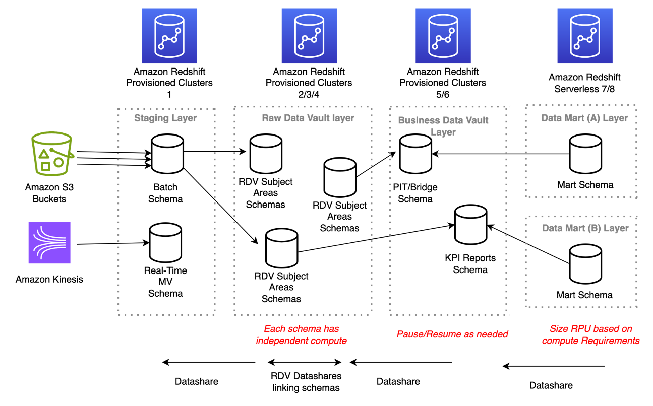
The following diagram illustrates the architecture for a large-scale Data Vault model.
Data Vault data model guiding principles
In this section, we discuss some recommended design principles for joining and filtering table access within a Data Vault implementation. These guiding principles address different combinations of entity type access, but should be tested for suitability with each client’s particular use case.
Let’s begin with a brief refresher of table distribution styles in Amazon Redshift. There are four ways that a table’s data can be distributed among the different compute nodes in a Redshift cluster: ALL, KEY, EVEN, and AUTO.
The ALL distribution style ensures that a full copy of the table is maintained on each compute node to eliminate the need for inter-node network communication during workload runs. This distribution style is ideal for tables that are relatively small in size (such as fewer than 5 million rows) and don’t exhibit frequent changes.
The KEY distribution style uses a hash-based approach to persisting a table’s rows in the cluster. A distribution key column is defined to be one of the columns in the row, and the value of that column is hashed to determine on which compute node the row will be persisted. The current generation RA3 node type is built on the AWS Nitro System with managed storage that uses high performance SSDs for your hot data and Amazon S3 for your cold data, providing ease of use, cost-effective storage, and fast query performance. Managed storage means this mapping of row to compute node is more in terms of metadata and compute node ownership rather than the actual persistence. This distribution style is ideal for large tables that have well-known and frequent join patterns on the distribution key column.
The EVEN distribution style uses a round-robin approach to locating a table’s row. Simply put, table rows are cycled through the different compute nodes and when the last compute node in the cluster is reached, the cycle begins again with the next row being persisted to the first compute node in the cluster. This distribution style is ideal for large tables that exhibit frequent table scans.
Finally, the default table distribution style in Amazon Redshift is AUTO, which empowers Amazon Redshift to monitor how a table is used and change the table’s distribution style at any point in the table’s lifecycle for greater performance with workloads. However, you are also empowered to explicitly state a particular distribution style at any point in time if you have a good understanding of how the table will be used by workloads.
Hub and hub satellites
Hub and hub satellites are often joined together, so it’s best to co-locate these datasets based on the primary key of the hub, which will also be part of the compound key of each satellite. As mentioned earlier, for smaller volumes (typically fewer than 5–7 million rows) use the ALL distribution style and for larger volumes, use the KEY distribution style (with the _PK column as the distribution KEY column).
Link and link satellites
Link and link satellites are often joined together, so it’s best to co-locate these datasets based on the primary key of the link, which will also be part of the compound key of each link satellite. These typically involve larger data volumes, so look at a KEY distribution style (with the _PK column as the distribution KEY column).
Point in time and satellites
You may decide to denormalize key satellite attributes by adding them to point in time (PIT) tables with the goal of reducing or eliminating runtime joins. Because denormalization of data helps reduce or eliminate the need for runtime joins, denormalized PIT tables can be defined with an EVEN distribution style to optimize table scans.
However, if you decide not to denormalize, then smaller volumes should use the ALL distribution style and larger volumes should use the KEY distribution style (with the _PK column as the distribution KEY column). Also, be sure to define the business key column as a sort key on the PIT table for optimized filtering.
Bridge and link satellites
Similar to PIT tables, you may decide to denormalize key satellite attributes by adding them to bridge tables with the goal of reducing or eliminating runtime joins. Although denormalization of data helps reduce or eliminate the need for runtime joins, denormalized bridge tables are still typically larger in data volume and involved frequent joins, so the KEY distribution style (with the _PK column as the distribution KEY column) would be the recommended distribution style. Also, be sure to define the bridge of the dominant business key columns as sort keys for optimized filtering.
KPI and reporting
KPI and reporting tables are designed to meet the specific needs of each customer, so flexibility on their structure is key here. These are often standalone tables that exhibit multiple types of interactions, so the EVEN distribution style may be the best table distribution style to evenly spread the scan workloads.
Be sure to choose a sort key that is based on common WHERE clauses such as a date[time] element or a common business key. In addition, a time series table can be created for very large datasets that are always sliced on a time attribute to optimize workloads that typically interact with one slice of time. We discuss this subject in greater detail later in the post.
Non-functional design principles
In this section, we discuss potential additional data dimensions that are often created and married with business data to satisfy non-functional requirements. In the physical data model, these additional data dimensions take the form of technical columns added to each row to enable tracking of non-functional requirements. Many of these technical columns will be populated by the Data Vault framework. The following table lists some of the common technical columns, but you can extend the list as needed.
| Column Name | Applies to Table | Description |
| LOAD_DTS | All | A timestamp recording of when this row was inserted. This is a primary key column for historized targets (links, satellites, reference), and a non-primary key column for transactional links and hubs. |
| BATCH_ID | All | A unique process ID identifying the run of the ETL code that populated the row. |
| JOB_NAME | All | The process name from the ETL framework. This may be a sub-process within a larger process. |
| SOURCE_SYSTEM_CD | All | The system from which this data was discovered. |
| HASH_DIFF | Satellite | A method in Data Vault of performing change data capture (CDC) changes. |
| RECORD_ID | Satellite
Link Reference |
A unique identifier captured by the code framework for each row. |
| EFFECTIVE_DTS | Link | Business effective dates to record the business validity of the row. It’s set to the LOAD_DTS if no business date is present or needed. |
| DQ_AUDIT | Satellite
Link Reference |
Warnings and errors found during staging for this row, tied to the RECORD_ID. |
Advanced optimizations and guidelines
In this section, we discuss potential optimizations that can be deployed at the start or later on in the lifecycle of the Data Vault implementation.
Time series tables
Let’s begin with a brief refresher on time series tables as a pattern. Time series tables involve taking a large table and segmenting it into multiple identical tables that hold a time-bound portion of the rows in the original table. One common scenario is to divide a monolithic sales table into monthly or annual versions of the sales table (such as sales_jan,sales_feb, and so on). For example, let’s assume we want to maintain data for a rolling time period using a series of tables, as the following diagram illustrates.

With each new calendar quarter, we create a new table to hold the data for the new quarter and drop the oldest table in the series. Furthermore, if the table rows arrive in a naturally sorted order (such as sales date), then no work is needed to sort the table data, resulting in skipping the expensive VACUUM SORT operation on table.
Time series tables can help significantly optimize workloads that often need to scan these large tables but within a certain time range. Furthermore, by segmenting the data across tables that represent calendar quarters, we are able to drop aged data with a single DROP command. Had we tried to perform the same DELETE operation on a monolithic table design using the DELETE command, for example, it would have been a more expensive deletion operation that would have left the table in a suboptimal state requiring defragmentation and also saves to run a subsequent VACUUM process to reclaim space.
Should a workload ever need to query against the entire time range, you can use standard or materialized views using a UNION ALL operation within Amazon Redshift to easily stitch all the component tables back into the unified dataset. Materialized views can also be used to abstract the table segmentation from downstream users.
In the context of Data Vault, time series tables can be useful for archiving rows within satellites, PIT, and bridge tables that aren’t used often. Time series tables can then be used to distribute the remaining hot rows (rows that are either recently added or referenced often) with more aggressive table properties.
Conclusion
In this post, we discussed a number of areas ripe for optimization and automation to successfully implement a Data Vault 2.0 system at scale and the Amazon Redshift capabilities that you can use to satisfy the related requirements. There are many more Amazon Redshift capabilities and features that will surely come in handy, and we strongly encourage current and prospective customers to reach out to us or other AWS colleagues to delve deeper into Data Vault with Amazon Redshift.
About the Authors
 Asser Moustafa is a Principal Analytics Specialist Solutions Architect at AWS based out of Dallas, Texas. He advises customers globally on their Amazon Redshift and data lake architectures, migrations, and visions—at all stages of the data ecosystem lifecycle—starting from the POC stage to actual production deployment and post-production growth.
 Philipp Klose is a Global Solutions Architect at AWS based in Munich. He works with enterprise FSI customers and helps them solve business problems by architecting serverless platforms. In this free time, Philipp spends time with his family and enjoys every geek hobby possible.
 Saman Irfan is a Specialist Solutions Architect at Amazon Web Services. She focuses on helping customers across various industries build scalable and high-performant analytics solutions. Outside of work, she enjoys spending time with her family, watching TV series, and learning new technologies.