Explore the semantic knowledge graphs without SPARQL using Amazon Neptune with Rhizomer

This is a guest post written by Roberto García, Associate Professor and Deputy Vice-rector for Research & Transfer at Universitat de Lleida, Spain.

In this post, we illustrate how to use the Rhizomer web application to interact with knowledge graphs available as semantic data from an Amazon Neptune instance through its SPARQL endpoint.

Neptune is a fast, reliable, fully managed graph database service to build and run applications that work with highly connected datasets. Rhizomer is an open-source web application for interactive exploration of semantic and linked data available from SPARQL endpoints, and is comprised of a backend (RhizomerAPI) and a frontend (RhizomerEye), licensed under the GNU GPL v3.0 license.

For detailed instructions on how to configure Rhizomer and Neptune, follow the step-by-step instructions in the GitHub repo.

Data analysis with Rhizomer

With Rhizomer, you can explore datasets by performing the three typical data analysis tasks: get an overview, zoom and filter, and view details.

Overview

With an overview, you get the full picture of the dataset. Rhizomer automatically generates a word cloud to provide an overview of the kinds of things in the dataset. This is the default overview mechanism because it works even if you don’t have a schema or ontology for the dataset that organizes the classes of things in the dataset hierarchically.

If an ontology is defined for the dataset, you can also use more structured overviews like tree maps.

You can also see an overview based on a network representation of the most common classes and how they’re connected.

Zoom and filter

After you select a class, Rhizomer generates a faceted view. It zooms in and allows filtering resources of the chosen type based on their properties. As with the previous step, this view is generated automatically, fully driven by the underlying data so it’s available even if you don’t have a schema. This also allows you to explore data that doesn’t fully comply with an existing schema, and highlights these inconsistencies during exploration to help you spot them.

Details

After zooming and filtering, you arrive at the resources of interest. All properties and values are shown for every selected resource. You can also browse linked resources. We plan for future improvements to include visualizations like maps or timelines.

Additionally, you can use Rhizomer to configure the datasets for exploration, selecting from the underlying Neptune instance the graphs to combine and analyze to generate interactive visualizations. You can even create graphs and load small datasets thorough Rhizomer. However, for bigger datasets, we recommend using the bulk loading mechanism in Neptune, which we explain in the GitHub repo.

DBPedia is an example of a large dataset available as semantic data. It’s a huge knowledge graph generated from Wikipedia, which makes it available as structured data. The English version of DBPedia describes more than 7.5 million things. It includes 1.23 million persons, 840,000 places (including 479,000 populated places), 3.4 million creative works (including 2.9 million images, 139,000 music albums, and 112,000 films), 286,500 organizations (including 55,500 companies and 54,000 educational institutions), 300,000 species, 6,108 diseases, and more.

We describe how you can use Rhizomer to explore the DBPedia dataset loaded into Neptune. For detailed instructions on how to set up Rhizomer and Neptune, see the GitHub repo which walks you through starting your own Neptune instance, loading DBPedia, and deploying Rhizomer on AWS to interact with the loaded data.

Explore DBPedia with Rhizomer

We deploy Rhizomer in an Amazon Elastic Compute Cloud (Amazon EC2) micro instance, as detailed in the GitHub repo, and load the DBPedia dataset into Neptune. After you configure Rhizomer to point to the Neptune instance, you can start exploring a big dataset like DBPedia without any prior knowledge about the content of the dataset and how the entities are described. The GitHub repo shows you how to load DBPedia into Neptune.

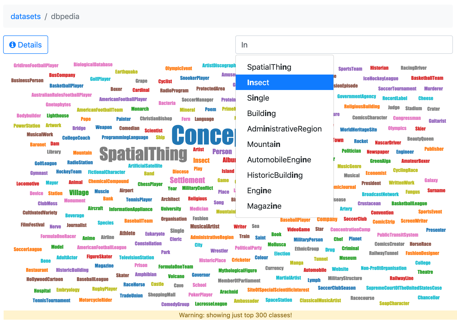
The first step when exploring a dataset like DBPedia is to generate the overview, which shows the 300 most common classes in the dataset. With this view, which is automatically generated, you can get an initial idea about the kinds of entities in the dataset and which ones are more represented.

Next, you can focus on the resources of interest. To do so, choose a word in the word cloud. If you have over 300 classes (as is the case with DBPedia), you can also search for a specific class. The search field includes an autocomplete feature to facilitate data discoverability. You just need to enter part of the class to view a list of possible matches.

The following overview of DBPedia is available online to explore.

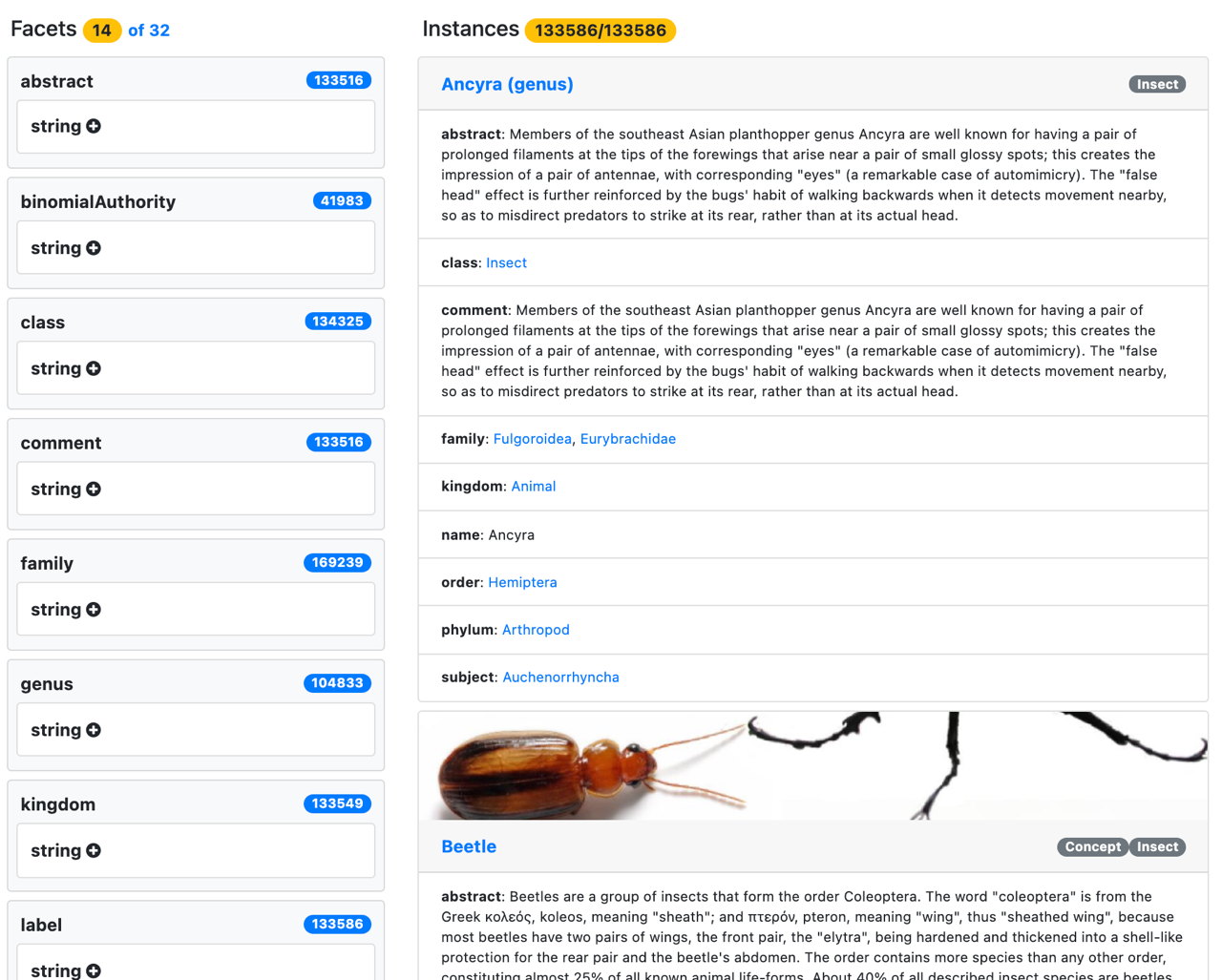
After you choose your class of resource (for example, insect), the faceted view for all 133,586 different insects in DBPedia is shown.

You can now use the list of facets to filter by attributes and relationships.

Filter by depiction

To demonstrate filtering by attributes, we filter just the insects with depictions by choosing depictions or the total count, which displays the number of depictions of insects.

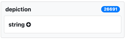
The depiction facet might not be visible initially because, to avoid a cluttered faceted view, just those facets most used are displayed first. You can choose the total number of facets to display them all.

A given insect may also have more than one depiction. This is evident, for instance, for subject. In this case there are more uses of this property (283,548) than insects (133,586), so we know some insects are classified into multiple subjects.

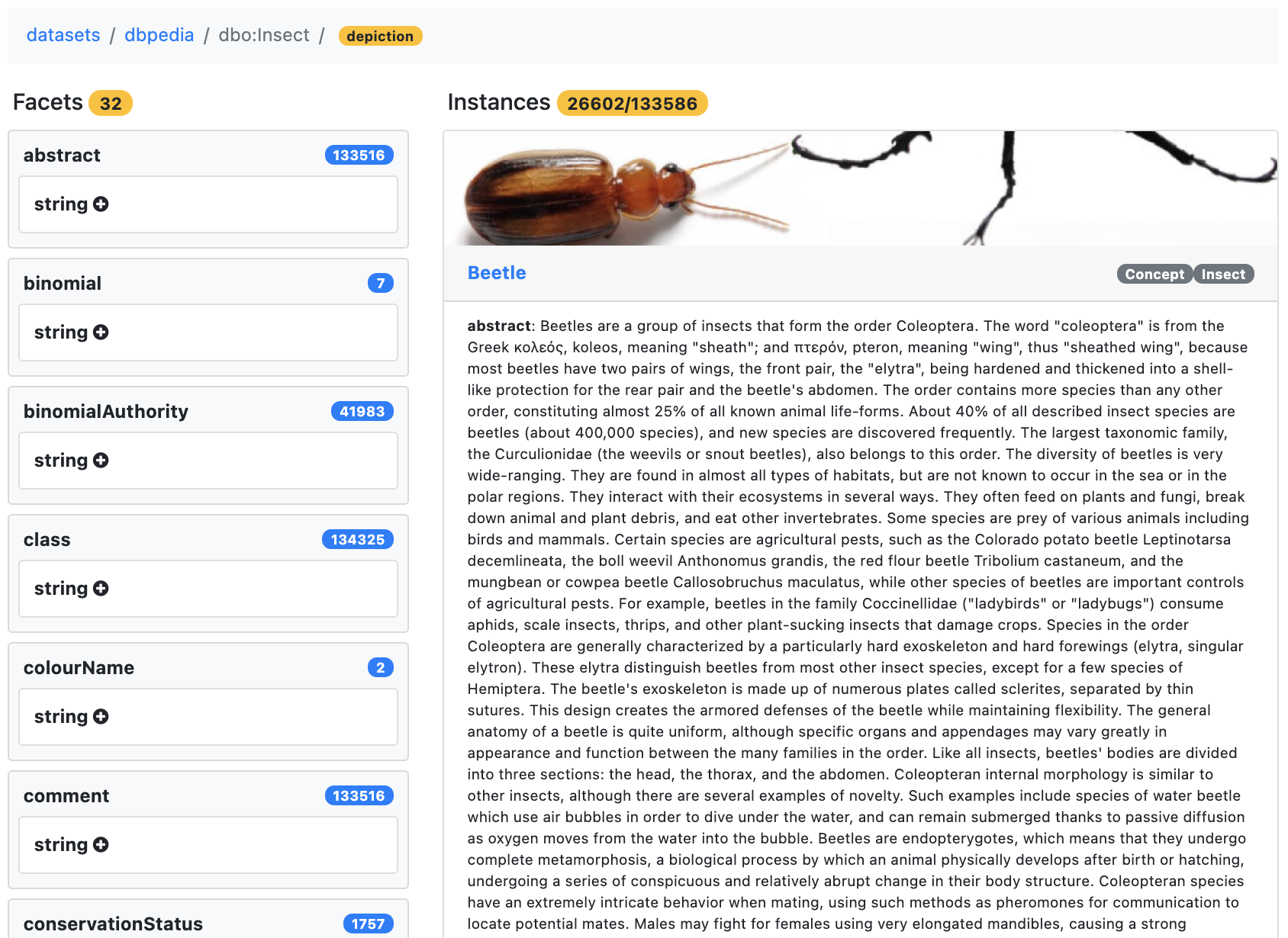
When you choose the depiction facet, it becomes orange to indicate that it’s selected.

The list of resources is updated to show just the resources with depictions, and you can see the applied filter on depiction.

Filter by common value

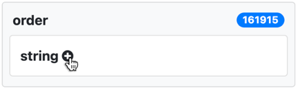
You can also use facets to list the 10 most common values for the selected resources with the filters applied so far. Choose the add icon next to the type of values for the facet. For example, we can choose the add icon next to string to under the order facet.

The 10 most frequent values for order for insects with depictions are displayed, along with the number of times they occur. The seventh most common value is Odonata, which you can choose in order to restrict the displayed entities to those in this order and depiction.

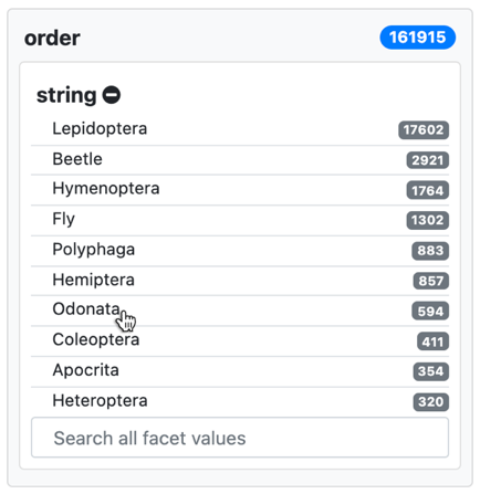
The selected order shows as highlighted and the list of resources is updated accordingly. The same happens for the facet values; the list of values reflects those for the selected resources. Now, Odonata appears as the most common value for order because the resources are limited to those with that value. The rest of values for the facet correspond to other additional values for order, which those also in Odonata might have.

Search for facets

To find values not among the most common for a facet, you can search for them. For example, you can search among the values for the facet subject for Insect with depiction and the order Odonata. When you expand the common values for the subject facet, you can see a search field. For example, you can list existing subject values containing dragon to use for further filtering.

View individual entries

As another way to view resource details, you can choose the title of an individual resource. For example, the following screenshot shows the details for Acisoma.

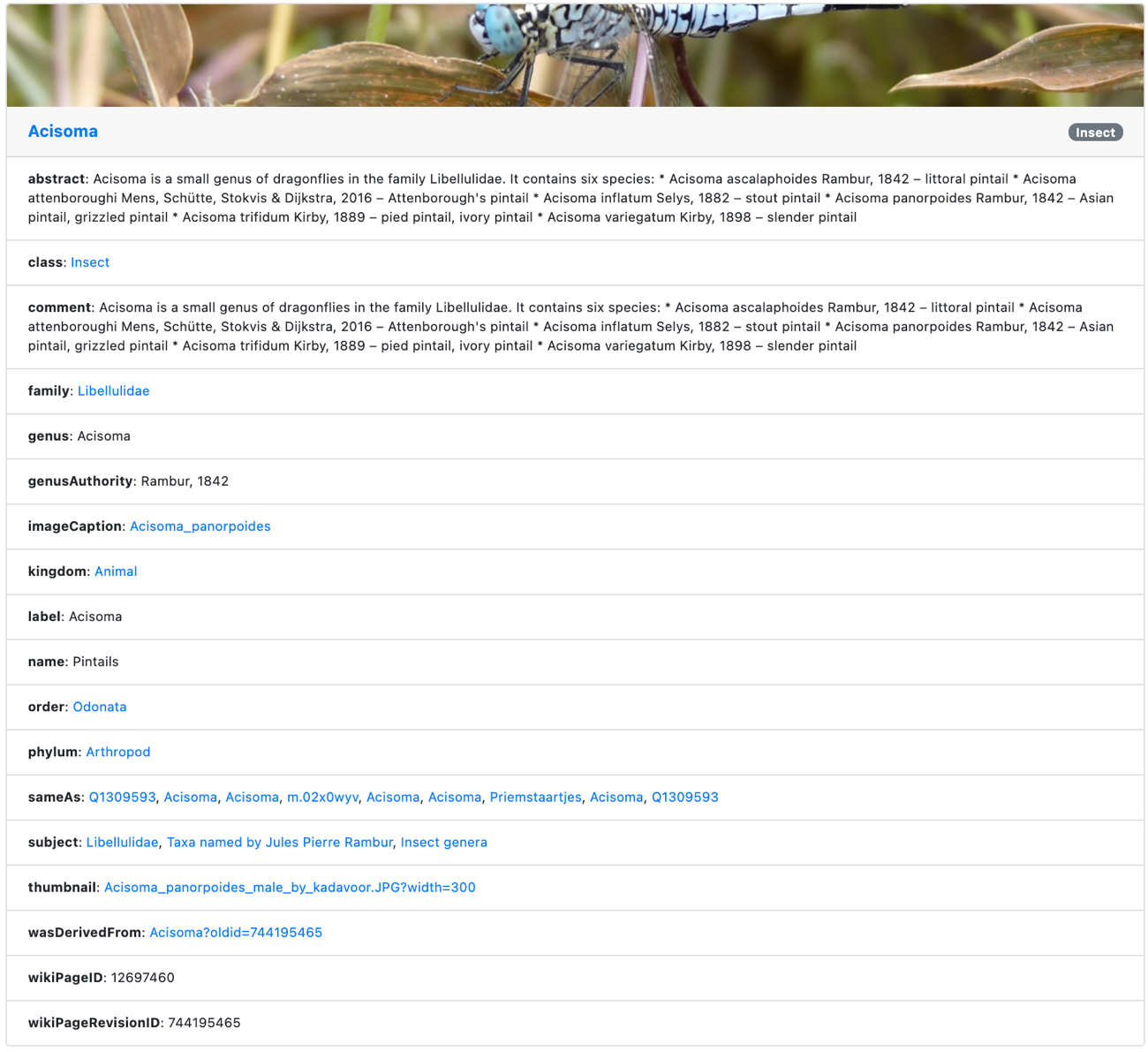
In this case, all the metadata for that resource is presented, including additional data that might be retrievable remotely from the URL identifying the resource. In our case, because not all DBPedia data has been loaded into Neptune (as detailed in the GitHub repo), additional data from the DBPedia entry on Acisoma is retrieved and combined with the local data.

The same mechanism works if you explore any link to a resource not loaded in Neptune. The linked data mechanisms check if remote data can be retrieved from the linked URL. If so, it’s included in your results, thereby making Rhizomer a linked data browser in addition to a tool to explore data loaded into a SPARQL endpoint like Neptune.

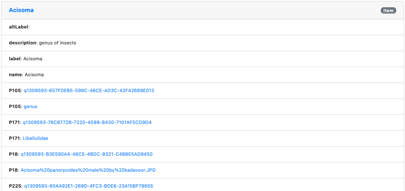
For instance, Acisoma is linked through a sameAs relationship to the equivalent entity in the Wikidata knowledge graph Q1309593. When you choose the corresponding link, the data is retrieved from the remote URL and shown in the results.

You can continue exploring through linked data resources and browse the corresponding remote resources. Alternatively, you can return to the data loaded in Neptune and continue exploring the overview, faceted views, and details.

Conclusion

Graph databases like Neptune and semantic data make it possible to create rich knowledge graphs that make data-driven applications possible. Rhizomer is an example of such an application. Without any preliminary configurations, Rhizomer automatically generates a user interface that allows you to explore an interactive knowledge graph. You don’t have to know a query language like SPARQL or understand the underlying schema followed by the data (such as vocabularies, ontologies, classes, properties, or their URIs).

Rhizomer facilitates exploring custom graphs in addition to existing knowledge graphs like DBPedia. This makes Rhizomer an ideal tool to validate your knowledge graphs as you build them in Neptune, or to explore third-party graphs to discover their structure and the value they can contribute to your projects.

Get started with Rhizomer and Neptune today by deploying the solution from the Rhizomer GitHub repo.

About the Author

Roberto García is Associate Professor and Deputy Vice-rector for Research & Transfer at Universitat de Lleida, Spain. He is also a part-time professor at the Next International Business School and a member of the Academic Advisory Board of the International Association for Trusted Blockchain Applications. He has more than 20 years of experience in research and innovation applying semantic technologies in different domains, especially in connection with knowledge and media management. More recently, he is exploring Web 3, as a combination of semantic and decentralization technologies like blockchain. He has applied Web 3, for instance, to facilitate social media monetization using Non-Fungible Tokens whose terms are modelled using a copyright ontology. To know more about him visit his home page.