Handle traffic spikes with Amazon DynamoDB provisioned capacity

If you’re using Amazon DynamoDB tables with provisioned capacity, one challenge you might face is how best to handle a sudden request traffic increase (spike) without being throttled. A throttle is a service response that occurs when DynamoDB detects your request rate has gone above a configured limit. For example, if you’ve provisioned a table for 10,000 write capacity units (WCUs), and it receives traffic at a rate that tries to consume 20,000, you will eventually start to see throttles, requiring those throttled requests to retry again to be satisfied.

The more sudden and extended the traffic spike, the more likely a table will experience throttles. However, throttles aren’t inevitable even for spiky traffic. Here we walk you through eight designs to handle traffic spikes, and present their advantages and disadvantages:

Utilize auto scaling and burst capacity
Adjust your auto scaling target utilization
Switch to on-demand mode
Have any background work self-throttle
Have any background work slow-start
If you can predict the spike timing, use an auto scaling schedule
If you can’t predict the spike timing, proactively request an auto scaling adjustment
Strategically allow some level of throttles

Background on DynamoDB throttles

With DynamoDB, there are two situations when read and write requests may be throttled. First, when the request rate to the table has exceeded the provisioned capacity of the table. Second, when the request rate to a partition has exceeded the hard limit present on all partitions. For this post, we focus on throttles at the table level. These are the limits most relevant to sudden traffic spikes.

To learn more about table and partition limits, see Scaling DynamoDB: How partitions, hot keys, and split for heat impact performance (Part 1: Loading).

With a DynamoDB provisioned table, you explicitly control the read and write abilities on the table by assigning provisioned throughput capacity. You assign a read throughput (in read capacity units, or RCUs) and a write throughput (in write capacity units, or WCUs). The more you allocate, the more read or write work the table or index can perform before throttling, and the higher the hourly cost.

Global secondary indexes (GSIs) have a provisioned throughput capacity separate from the base table. Their limits work exactly the same as on tables. In the remainder of this post, the term table can refer to both tables and indexes.

1. Utilize auto scaling and burst capacity

Traffic often fluctuates throughout the day, and the classic way to handle this with provisioned capacity tables is to turn on the auto scaling feature. Auto scaling observes the consumed capacity on a table and adjusts the provisioned capacity up and down in response. You configure a minimum (don’t go below this), a maximum (don’t go above this), and a target utilization (try to keep the amount being consumed as this percentage of the total amount provisioned). Auto scaling adjust to handle the usual end-user traffic variances and spikes throughout the day.

Auto scaling adjusts the provisioned capacity upward if it observes 2 consecutive minutes of consumed capacity above the target utilization. It adjusts provisioned capacity downward if it observes 15 consecutive minutes where the utilization is more than 20% (as in 2,000 basis points, not relative) under the target utilization line. Scaling up can happen at any time. Scaling down has more stringent rules, as explained in Service, account, and table quotas in Amazon DynamoDB:

“There is a default quota on the number of provisioned capacity decreases you can perform on your DynamoDB table per day. A day is defined according to Universal Time Coordinated (UTC). On a given day, you can start by performing up to four decreases within one hour as long as you have not performed any other decreases yet during that day. Subsequently, you can perform one additional decrease per hour as long as there were no decreases in the preceding hour. This effectively brings the maximum number of decreases in a day to 27 times (4 decreases in the first hour, and 1 decrease for each of the subsequent 1-hour windows in a day). Table and global secondary index decrease limits are decoupled, so any global secondary indexes for a particular table have their own decrease limits.”

Auto scaling uses Amazon CloudWatch to observe the consumed capacity. CloudWatch metrics aren’t immediate; they have a delay of 2 minutes or more. This means auto scaling is always looking a little into the past when watching a DynamoDB table. Auto scaling requires seeing 2 consecutive minutes of elevated requests for it to decide to raise the provisioned amount. This means the time from when a traffic surge begins until auto scaling has the data required to initiate a change will be 4 minutes at minimum.

The target utilization feature of auto scaling provides padding designed to accommodate traffic spikes during this time window. If your table is consuming 70,000 WCUs, auto scaling with a 70% target utilization will provision 100,000 WCUs. The extra 30,000 WCUs are padding to handle traffic spikes until auto scaling can provision higher. This keeps all but the most extreme spikes in traffic from seeing throttles.

When there are spikes that exceed the padding, DynamoDB offers burst capacity, which allows tables to temporarily exceed their provisioned levels, up to a finite amount. For more information, refer to Scaling DynamoDB: How partitions, hot keys, and split for heat impact performance (Part 2: Querying). Burst capacity is always enabled.

Figure 1 shows typical auto scaling behavior. The jagged orange line is the consumed write traffic fluctuating throughout the day from 300,000 to 650,000 WCUs. The horizontal blue lines are the provisioned write capacity as controlled by auto scaling. It goes up and down in reaction to the need.

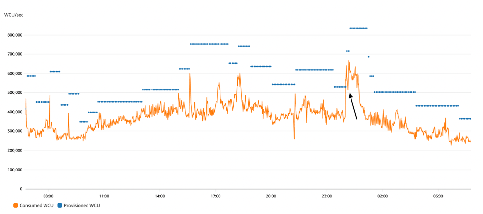
Figure 1: Autoscaling behavior: the jagged orange line is write consumption and horizontal blue lines are provisioned capacity

Right after midnight (three quarters of the way into the graph), if we look carefully, we can see the effects of throttling. The orange consumption line jumped dramatically from 375,000 WCUs to 640,000 WCUs, well over the blue provisioned capacity line set at 520,000 WCUs. This temporary excess was allowed due to burst capacity. The spike persisted and after a few minutes the burst capacity was exhausted, causing the orange consumption line to come back down to the provisioned line for about a minute before auto scaling was able to raise the blue provisioned line upward, letting consumption rebound. (The black arrow points at this event.)

Figure 2 shows an hour-long synthetic test designed to generate throttles, jumping the user load from 4,000 WCUs to 18,000 WCUs. This synthetic test includes random jitter like true user load but it’s all artificially generated so we can tweak various behaviors and test the result.

The table for this first test has auto scaling enabled with a 70% target utilization. The top of the diagram shows the resulting consumed capacity (the fluctuating blue line) as well as the provisioned capacity (the squared red line). The bottom of the diagram shows the throttle count on the table during the same time frame. The spike is steep and long enough to cause throttles.

Disclosure: the red line has been hand drawn to show the minute-by-minute scaling activities exactly as described in the auto scaling event log. CloudWatch does not receive provisioned capacity information at minute level of granularity.

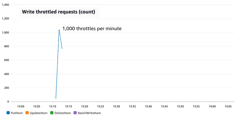
Figure 2: A synthetic test showing a sudden jump in traffic from 4,000 to 18,000 WCUs on a table with auto scaling configured with a 70% target utilization

The test starts with fairly flat traffic consuming 4,000 to 5,000 WCUs. Auto scaling keeps the provisioned capacity floating at around 7,500 WCUs. Simple fluctuations in traffic are handled by the padding. Then at 13:07 the write traffic immediately jumps to 18,000 WCUs. Initially there are no throttles. Burst capacity permits the excess usage. At 13:11, however, the burst capacity runs out and the write rate goes down to the provisioned amount, with all other requests throttled. The throttling continues until 13:13 when auto scaling grows the provisioned capacity up to 26,000 WCUs, enough to handle the spike and with padding as well in case there’s another. Finally, about 15 minutes after the spike has subsided, auto scaling drops the provisioned amount back down.

The rest of this post examines designs when you have tables with access patterns including extremely sharp and sustained read or write traffic growth scenarios like this beyond what default auto scaling can handle.

2. Adjust your auto scaling target utilization

One adjustment to consider is to set your auto scaling target utilization lower. This works well if you’re getting end-user traffic spikes at times you can’t anticipate and want to maintain low latency by avoiding throttles.

The auto scaling target utilization controls how much padding your table keeps on hand for handling spikes. It can range from 20% to 90%. Lower values mean more padding. A target of 40% will allocate 1.5 times the current traffic level to padding, so a table actively consuming 10,000 WCUs would provision 25,000 WCUs to achieve that 40% target. A lower target utilization has three benefits:

It provides more padding to handle spikes.
It increases the burst capacity allowance should the spike go above the provisioned level, because the burst capacity allowance is proportional to the provisioned amount.
It allows auto scaling to ramp up faster. Auto scaling looks at how much consumed capacity has exceeded the target utilization to decide how much to increase. It doesn’t look at throttle counts. If you have more padding, then more of the unexpected spike can be seen and used to calculate a large jump. If you have very little padding, the spike will appear more muted (instead of consuming capacity, it produces throttles), and auto scaling will step up with smaller steps.

The downside is increased cost. You’re charged based on the provisioned amount, so more padding means more cost. Also, every time auto scaling adjusts provisioned capacity upward in response to the traffic spike, it might have to wait some time to adjust downward again. More padding adds extra cost during that time too. Choosing the right target utilization is a balancing act between throttles and cost.

If you choose to adjust the auto scaling target utilization, don’t forget to consider the GSIs as well as the base table.

Figure 3 recreates the same traffic pattern as earlier, but now using a target utilization of 60%. It has no throttles.

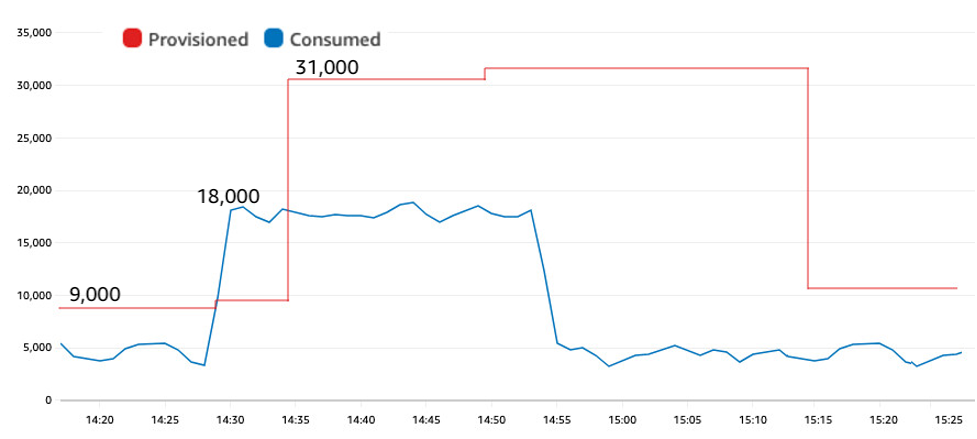
Figure 3: A synthetic test showing a sudden jump in traffic from 4,000 to 18,000 WCUs on a table with auto scaling configured with a 60% target utilization, now without throttles

The lower target utilization provided more padding. During the first 10 minutes of the test, auto scaling provisioned closer to 9,000 WCUs instead of 7,500 WCUs as in the previous test. The jump to 18,000 WCUs happened at 14:28 and at 14:35 auto scaling adjusted the provisioned amount upward. Despite the same significant spike as in Figure 2, the table with a lower target utilization experienced zero throttles.

The lower target utilization provided two benefits here: First, extra padding meant less burst capacity was required during the spike. Second, having a higher provisioned amount ahead of the spike meant more burst capacity was available to consume. That combination eliminated any throttles for this scenario.

3. Switch to on-demand mode

A useful design to consider if avoiding throttles is paramount is to change the table to on-demand mode.

With on-demand, pricing is based wholly on consumption. Each request incurs a small charge. Instead of allocating a certain amount of RCUs and WCUs per second and paying by the hour, you simply consume read request units (RRUs) or write request units (WRUs) each time you make a request. With on-demand, there is no provisioning and there’s no need for auto scaling, up or down. It’s ideal for spiky workloads and unpredictable workloads.

An on-demand table greatly reduces the likelihood of throttles in response to sudden traffic spikes. An on-demand table throttles only for two reasons. First, if a partition’s limits are exceeded (same as provisioned). Second, if the traffic to the table exceeds the account’s table-level read or write throughput limits, which both default to a soft guardrail of 40,000 but can be set higher and there is no extra charge for them being set higher.

Figure 4 recreates the same traffic pattern, but now on a table in on-demand mode. There is no provisioned value (no red line) and no table-level throttles.

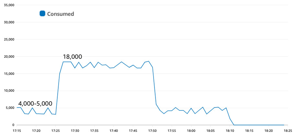
Figure 4: On-demand reacts immediately to spikes in traffic without throttling

Converting your table to on-demand is the “set it and forget it” choice. There’s no need to think about provisioning, target utilization, upscaling, or downscaling. You can convert a table back and forth between provisioned and on-demand. Tables can be switched to on-demand mode once every 24 hours. Tables can be returned to provisioned capacity mode at any time. You might find it useful to convert a table to on-demand for the times each day when you anticipate spikes, then convert to provisioned for the other smoother traffic time periods.

There’s a common misconception that on-demand tables are more expensive than provisioned tables. Sometimes yes, sometimes no. For relatively flat traffic, provisioned will be superior in terms of cost. The more the workload has traffic spikes (sharp rises and falls), the more cost advantageous on-demand becomes. With enough spikes, it can become the lower-cost option. That’s because on-demand avoids all extra costs around padding, and there’s no waiting for downsizing after a spike.

Mathematically, if the achieved utilization on a provisioned table is below 15%, on-demand will be a lower-cost option. Achieved utilization is calculated as the sum of consumed capacity divided by the sum of provisioned capacity over the month. It’s lower than the target utilization because of the delay in downsizing.

4. Have any background work self-throttle

If your traffic spikes are caused by background actions where you have some control, you have another option to consider, which is to have the background activity self-throttle. Basically, have the background action restrict its consumption rate so it doesn’t compete excessively with end-user traffic, and also so it dampens the necessary auto scaling increases.

Significant spikes often come about because of some background activity: loading new datasets, a daily item refresh, selectively deleting historic data, or scanning a table for analytics. In these situations, you might have some control on how the background work behaves.

You can have the background task run at some self-limiting rate. Choose a rate designed to easily fit within the usual auto scaling padding. That way, it won’t cause throttles when it starts (assuming no hot partitions), and auto scaling can adjust upward to restore the necessary padding on the table. If it’s an external party driving the spiky traffic, consider if you could rate-limit each external party at their application access point.

The bulk work can self-limit by asking for ReturnConsumedCapacity on each of its requests and tracking how much capacity it’s consuming per second. If too high, it can slow down. In the likely event you’re using multiple separate client processes, you might allow a certain max capacity consumption rate per client.

The following figure shows how self-throttling bulk work can limit the size of the spike and avoid throttles. The table has a 70% target utilization again same as in Figure 2, but now the request rate jumps to 14,000 WCUs only, because the bulk processing task has been redone to run a bit slower for a bit longer.

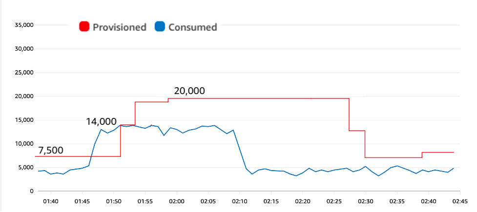
Figure 5: Jumping to 14,000 WCUs instead of 18,000 eliminates throttles

The smaller spike to 14,000 WCUs results in less burst capacity consumed during the spike, and gives auto scaling time to adjust upward before the table experiences throttles

The self-throttle approach works if it’s acceptable for the background work to run at a moderated pace. If so, it has the extra advantage that it limits how much the auto scaling will adjust upward. Imagine you have background work that can consume a steady 4,000 WCUs for 10 minutes or 8,000 WCUs for 5 minutes. With an on-demand table, these two options are priced the same. With a provisioned table using auto scaling, the more moderated job will cause a smaller auto scaling increase. If the auto scaling decrease has to wait an hour, that’s an hour at much lower provisioned capacity. For the test results here, you can see the peak provisioned was 20,000 WCUs, down from 26,000 WCUs in the original test.

This approach turns spikes into plateaus—and any plateaus with auto scaling tend to be lower cost.

5. Have any background work slow-start

If you have background work that you want to complete as quickly as possible and don’t want to risk causing throttles that impact end-user traffic, you can have the background work slow-start.

A slow-start requires the work self-throttle as stated earlier, but only starts slow then increases the request rate every few minutes. This easing-in behavior gives auto scaling time to adjust to the increased demand for capacity. As with sports, you want to warm-up first to avoid breaking anything.

Compared to the previous option, this doesn’t provide a potential cost savings, but it does limit the risk of table-level throttles and competition with end-user traffic, while allowing for (after warming up) an arbitrarily rapid request rate (limited only by your configured auto scaling maximum and account-level and table-level limits).

The following figure shows how a slow-start was able to fit within the auto scaling padding to avoid throttles while also sending signals to auto scaling about the need to increase capacity.

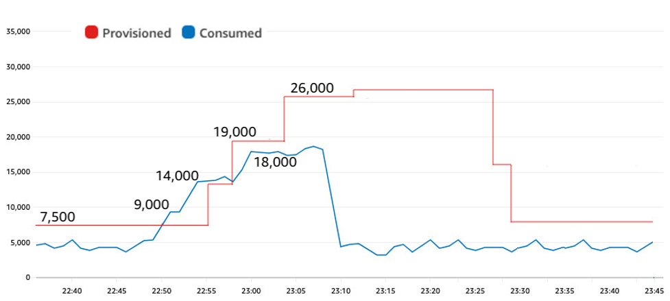
Figure 6: A slow start to the background processing allows auto scaling time to adapt

The traffic grew in steps: from 4,000 to 9,000 to 14,000 and then to 18,000 between 22:49 and 23:00. This slow-start gave auto scaling time enough to react with its own series of increases before the burst capacity was depleted. The test reached the same 18,000 WCUs rate as in the original test, with the same 70% target utilization, yet by starting slow it avoided all throttles.

6. If you can predict the spike timing, use an auto scaling schedule

If you have spikes and they’re predictable—for example, every day at 5:00 AM you do a bulk load, or every morning at 9:00 AM end-user requests go from non-existent to rapid-fire—you can use scheduled scaling.

With scheduled scaling, you’re able to set different values for your table’s minimum and maximum depending on the day and time. You have the full expressiveness of crontab in controlling the scheduled actions.

For example, if you know a spike is coming and its size, you could change the autoscaling minimum settings to be large enough to handle the spike, which will push the table’s provisioned capacity up. You can drop down the minimums once the spike starts. Dropping the minimum doesn’t drop the provisioned amount, it only allows auto scaling to drop it when it actually sees the reduced consumption.

The following figure shows a scheduled action that adjusted the auto scaling minimum to 18,000 WCUs two minutes before the spike in traffic jumped to that rate.

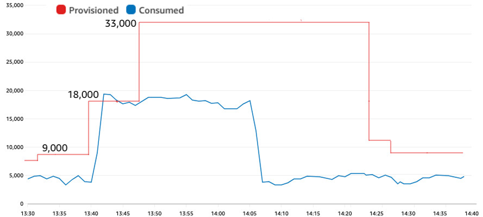
Figure 7: Proactively scaling up before a predictable spike

This proactive adjustment of the auto scaling minimum avoided any throttles. The first raise to 18,000 was the scheduled action. The second raise to 33,000 was auto scaling responding to the actual traffic and adding the necessary padding.

7. If you can’t predict the spike timing, proactively request an auto scaling adjustment

If instead you have spikes where you can’t anticipate the exact timing, but you can detect when they’re about to start, you can directly force an auto scaling adjustment proactively.

For example, maybe you know that there will be a bulk load in the morning but you don’t know exactly when. You can have the bulk load proactively request a specific capacity raise as it’s beginning. Imagine it making a “Get ready, here I come” call for a certain capacity amount, and the table can adjust without delay.

It’s actually quite quick to adjust a table’s provisioned capacity upward, once the call has been made to do so. It takes less than a minute usually. The one caveat is if you raise a table’s provisioned limit higher than it had ever been set previously. If you set a new high-water mark like this, it might be necessary for the table to grow its capability, and this growth can take time. A best practice is to establish the high-water mark in advance by one time provisioning the table and indexes to the maximum read and write levels needed in production before downscaling again. That ensures that later capacity raises can be quickly achieved. If you can do this upon table creation, that’s fastest.

Now let’s discuss how to proactively increase an auto scaling table’s provisioned capacity. If you directly update the table, auto scaling won’t know about the change, and could undo your change with its own auto scaling action. The more reliable technique is to adjust the auto scaling minimum to be what you want as the new provisioned capacity. That way auto scaling does the raise for you and is aware it happened.

Each requester of capacity should go to a coordinator, request a certain amount of additional capacity be added to a table or GSI, wait for it to be fulfilled, and then start without delay and without causing table-level throttles.

The coordinator receives each request, examines the current traffic, adds the requested amount, and assigns a new auto scaling minimum. After a few minutes, it can adjust the minimum back to the original value, trusting that the bulk worker’s activity will keep the provisioned level at the higher requested amount until the bulk work ends. There’s no need to carefully time the downscale. It’s only necessary to quickly upscale the table.

The end result looks and behaves the same as Figure 7, with the only change that you don’t need to know the timing in advance.

8. Strategically allow some level of throttles

One final design to consider is to strategically allow throttles in your application design. Consider this if reliably low latency isn’t a hard requirement. Accepting some throttles can be a cost-effective choice.

Throttles aren’t catastrophic. They don’t cause any database damage. They just increase latency.

For example, if you’re performing a bulk load on a table that doesn’t have concurrent end-user traffic, then it might be just fine for the bulk load to run just at or above the maximum capacity of the table with some throttles happening along the way. It means the load will take a little longer than if the capacity was raised to eliminate the throttles, but the cost will be flat and every bit of capacity will get used, no padding or other considerations needed.

However, if the table has concurrent end-user traffic, then running a bulk load like this will cause end-users to see throttles with their writes as well, increasing their perceived latency, and that might be a problem. The choice to strategically allow throttles works best when no clients require low latency.

Note that SDK calls by default retry requests again if they see a throttle response. You often won’t be aware of this happening because it’s done within the SDK itself. A request might be retried a few times and then succeed and it would look to the client like a successful (but higher than usual latency) request. Only if the SDK has failed enough times to exceed the SDK’s configurable retry count do you see a provisioned throughput exceeded exception. If you see this exception, you should catch the exception and (assuming you still need the work done) try the request again. Eventually, the request will succeed. If your table is provisioned at 10,000 RCUs, then every millisecond there’s 10 more RCUs available for request handling.

Throttle events appear within CloudWatch as ReadThrottleEvents, WriteThrottleEvents, and ThrottledRequests. A small number of throttled clients can generate a large number of throttle events when the clients perform a series of quick automatic retries before succeeding. For this reason, you should focus on the general relative magnitude of the throttle events rather than the exact count. Also, remember that throttles can occur at the table level, but they can also occur at the partition level if you have hot partitions. CloudWatch metrics do not differentiate between the two, although CloudWatch Contributor Insights can help debug this.

Conclusion

Auto scaling and burst capacity can handle significant traffic spikes, but the more sudden and extended the spike, the more likely a table will experience throttles.

You can adjust the auto scaling target utilization downward, which allows more headroom for traffic growth, or you can change the table to on-demand mode, a set it and forget it choice.

If the surge is caused by background work (as large and sustained surges often are) you can have the background work self-throttle to keep its consumption low, or have it start slow before growing to full speed give auto scaling time to adapt.

If you know in advance the time when the surge is coming, you can schedule an auto scaling change to raise the throughput minimum enough to handle the surge. If you don’t know the surge timing in advance but can identify a starting moment, then you can proactively request the auto scaling increase.

Lastly, if low latency isn’t required, you might decide to strategically allow some level of throttles.

When making changes, don’t forget to adjust any GSI settings as well.

If you have any comments or questions, leave a comment in the comments section. You can find more DynamoDB posts and others posts written by Jason Hunter in the AWS Database Blog.

About the authors

Jason Hunter is a California-based Principal Solutions Architect specializing in Amazon DynamoDB. He’s been working with NoSQL databases since 2003. He’s known for his contributions to Java, open source, and XML.

Puneet Rawal is a Chicago-based Sr Solutions Architect specializing in AWS databases. He holds more then 20 years of experience in architecting and managing large-scale database systems.