AWS Database Blog
Use virtual partitioning in the AWS Schema Conversion Tool
The AWS Schema Conversion Tool (AWS SCT) is a general purpose tool to help you migrate between database engine types. For example, you can use AWS SCT to migrate an Oracle schema to Amazon Aurora PostgreSQL. AWS SCT is a free download available on the AWS website. You can install AWS SCT on any Windows, Fedora, macOS, or Ubuntu server that has access to your source and target databases.
For data warehouse migrations, AWS SCT not only helps you migrate your database schemas to Amazon Redshift, it can also migrate your data. The AWS SCT data extractors extract your data from an Oracle, Microsoft SQL Server, Teradata, IBM Netezza, Greenplum, or Vertica data warehouse and upload it to Amazon S3 or Amazon Redshift. The AWS SCT data extractors are a free download and can be installed on any of the same platforms as AWS SCT.
In this post, we look at how to use virtual partitioning to optimize your data warehouse migrations using AWS SCT. Virtual partitioning speeds up large table extraction using parallel processing. It is a recommended best practice for data warehouse migrations.
Data migration strategies in AWS SCT
A common question that we get from customers is about how they can tune the AWS SCT data extractors to speed up their database migrations. In a data warehouse environment, which can contain archival information, it’s likely that you have a great disparity in table sizes—some big, some small, and many in between. You can configure multiple AWS SCT extractors, each of which can extract and load multiple tables in parallel. However, the largest tables in the source database will still dominate the overall migration timeline.
Therefore, it is advantageous from a performance perspective to partition the large tables into smaller chunks that can be migrated in parallel. AWS SCT provides two mechanisms to accomplish this. If your tables are physically partitioned in the source (for example, using range partitioning in an Oracle database), AWS SCT migrates the table on a partition basis automatically using the UNION ALL VIEW system option.
If your source tables are not partitioned, you can use AWS SCT to create virtual partitions. Virtual partitions decrease your migration timeline by parallelizing the extraction of large source tables. In a nutshell, virtual partitioning is a divide-and-conquer approach to migrating large tables. Partitions can be migrated in parallel, and extract failure is limited to a single partition instead of the entire table. Using virtual partitioning is a recommended best practice for data warehouse migrations using the AWS SCT extractors.
You might be curious about what happens “under the hood.” AWS SCT creates a subtask for each table partition, physical or virtual. Then, when the migration is running, AWS SCT assigns the subtask to an available data extractor to execute. Essentially, AWS SCT orchestrates which subtask executes on which extractor, thereby keeping all extractors as busy as possible throughout the migration.
As with many technologies, it helps to understand how a feature works and its inherent tradeoffs in order to use it effectively. In the rest of this post, we walk through some examples to explain how virtual partitioning works. Then we describe a methodology that you can use to choose partitioning keys for your tables.
Before doing that, let’s briefly review what virtual partitioning is and how to use the feature.
Types of virtual partitioning
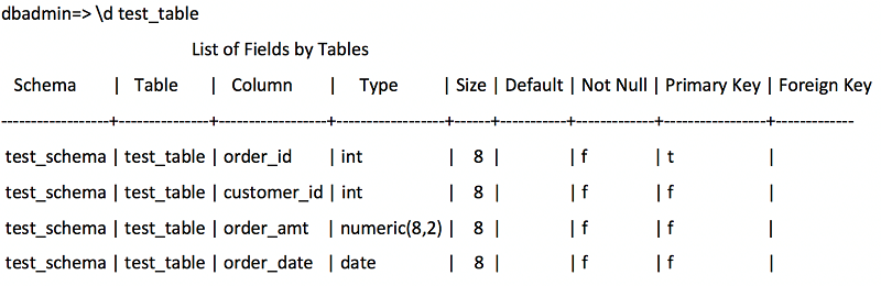
AWS SCT provides three types of virtual partitioning: list, range, and auto split. In this section, we describe each type of partitioning. We use the following Vertica source table as an example throughout.
List partitioning
List partitioning creates partitions based on a set of values that you specify. One partition is created for each value. If you choose, AWS SCT can also create a catch-all partition for all rows that are not covered by a listed value.
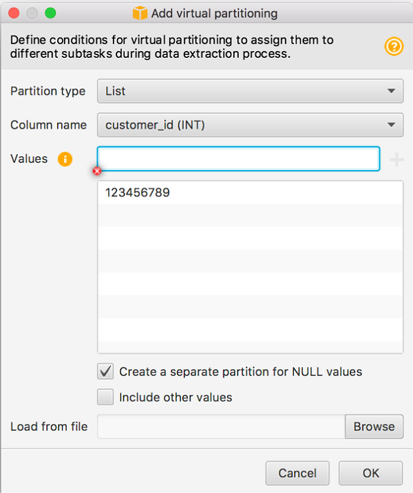
For example, the following screenshot shows list partitioning being applied to the CUSTOMER_ID attribute in AWS SCT.
You can switch to the Virtual partitions tab in AWS SCT to see the generated partitions. Choose the table name in the upper-middle pane to display the partitions.

Note that a partition is created for records with CUSTOMER_ID = 123456789. Because we selected the Create a separate partition for NULL values check box, a second partition is created to capture those rows. Any rows that do not match either of these conditions are filtered out of the migration. This is one advantage of list partitioning: You can use it if you only want to migrate a subset of the data to the target.
Otherwise, you can create a catch-all partition by selecting the Include other values check box.
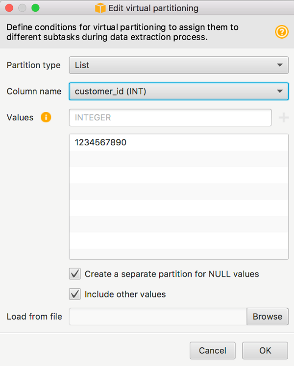
The catch-all partition is created using a NOT IN condition. You can switch to the Virtual partitions tab in AWS SCT to see the partitions.
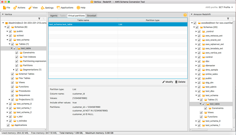
As noted earlier, when the table is migrated, three subtasks are created—one for each partition.
Range partitioning
Range partitioning creates partitions that correspond to ranges of values. You specify a list of values, and AWS SCT sorts those values and then creates partitions based on adjacent values. For example, you can use range partitioning to create partitions on ORDER_DATEs, as follows.

Notice that the partitioning values were loaded from a file, as shown in the Load from file field. This is a convenient way to create partition values, especially for large lists that might have tens or hundreds of values. Load from file is available for both list and range partition types. As before, you want to capture any rows with NULL values in the partitioning attribute by selecting the Create a separate partition for NULL values check box.
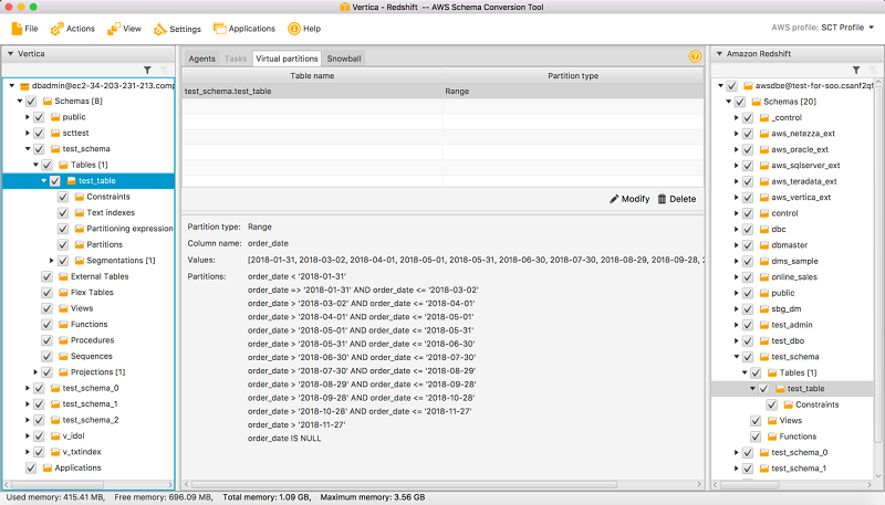
For range partitioning, by default, AWS SCT creates catch-all partitions at “both ends” of the specified partition values. With range partitioning, all source data is migrated to the target; you cannot filter the data as you can with list partitioning.
Date fields are usually good candidates for range partitioning.
Auto split partitioning
Auto split partitioning is an automated way of generating range partitions. With auto split, you tell AWS SCT the partitioning attribute, where to start and where to end, and how big the range should be between the values. Then AWS SCT calculates the partition values automatically.
For example, you can use auto split to create weekly partitions as follows.

As noted earlier, you can review the generated partitions on the Virtual partitions tab.
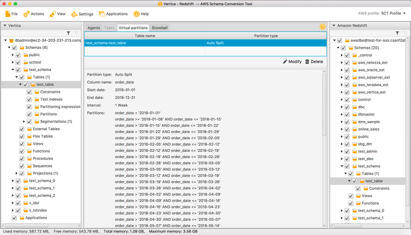
Auto split automates a lot of the work that is involved with creating range partitions. The tradeoff between using auto split and range partitioning is how much control you need over the partition boundaries. Auto split always creates equal size (uniform) ranges. With range partitioning, you can vary the size of each range. For example, the range can be daily, weekly, biweekly, monthly, etc., as needed for your particular data distribution. Another difference is that auto split always includes a partition for NULL values, but you have to specifically select this option for range partitioning.
Auto split partitioning is the default choice when choosing date/time attributes for virtual partitioning. It simplifies the range partitioning process by eliminating the need to specify the individual partition boundaries. However, you relinquish some control over the partitioning because the partition granularity is a uniform size. For example, look at the orders table mentioned earlier. If sales volumes are seasonal, peaking in the fourth quarter of the year, then auto split preserves some of the data skew no matter the partition granularity.
In most customer migrations, range partitioning and auto split partitioning are the preferred partitioning methods. This is because most large tables tend to be transactional tables and therefore have timestamps or datestamps that can be used as partitioning attributes. Or, they are large dimensional tables with sequence-based key values that can be used.
For the rest of this post, the examples concentrate on range partitioning. Because auto split partitioning is a shortcut for creating range partitions of uniform size, the same conclusions apply to auto split partitioning.
Test environment
We’ll use the test_table described earlier as an example table. We created this table in a single node Vertica 9 database and loaded it with 100 million records. The ORDER_ID field was populated as a sequence-generated integer in the range of [0 to 100 million]. Put differently, the ORDER_ID field has a uniform distribution in the given range of values.
The other relevant data distributions are shown in next two figures. The following table shows the order count by customer.
| # of customers | order count |
| 475973 | 0–100 |
| 428816 | 101–150 |
| 23645 | 151–200 |
| 21574 | 201–250 |
| 756 | 251–300 |
| 763 | 301–350 |
| 30 | 351–400 |
| 24 | 401–450 |
| 2 | 451–500 |
| 1 | 501–550 |
The following figure shows the skewed attribute distribution. In this chart, the order volume is seasonal, with the lowest activity in Q1 and peak activity in Q4.
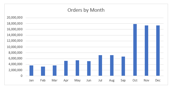
Skewed data such as this can have a negative impact on migration performance, depending on how the virtual partitioning is configured. For example, if a simple monthly partition is used, then the last three months of the year will dominate the overall migration performance. In the following section, we dive into best practices to mitigate the effects of data skew.
Using range partitioning
To demonstrate virtual partitioning, we first generated a benchmark timing without partitioning and then ran a series of migrations with increasingly granular partitioning. The partition values were generated using a Python program and then loaded into AWS SCT using the Load from file feature described earlier. For all tests, we created “extract only” tasks. That is, the task performed the data extract from Vertica to local storage, plus any file operations, including file chunking and compression. The tasks did not perform any downstream operations such as upload to Amazon S3 or COPY into Amazon Redshift.
Uniform data distributions
We first look at how range partitioning performs on uniformly distributed data. This is in some respects the “best-case” scenario. The results are shown in the following chart.
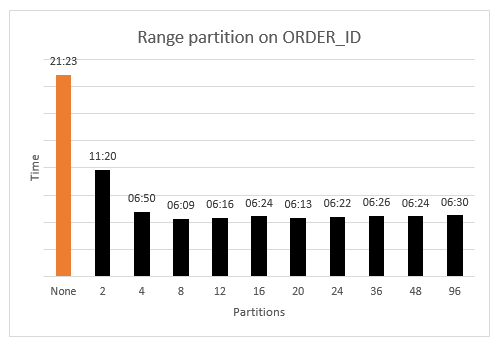
The benchmark “no-partitions” timing is shown in orange (on the far left side). The black bars show the timings for increasing partition granularity. As the chart shows, any partitioning is beneficial versus no partitions. Even with two partitions, the worst-case performance is nearly halved (11:20 vs. 21:23).
Another thing to note is that nearly optimal performance is achieved at a fairly low number of partitions (between 8 and 12). Beyond this granularity, performance is essentially flat, with a small increase at higher partitions due to task management within AWS SCT.
Because the ORDER_ID data is uniformly distributed over the data domain (integers between 0 and 100 million), each partition is guaranteed to be of nearly equal size. Attributes with uniform distribution are excellent candidates for range partitioning, and you can achieve efficient partitioning at fairly low granularity. In this case, there is no compelling reason to over-partition the data. For uniform data, a few experiments with low/medium partition granularity should be sufficient to find the “sweet spot” that balances performance and the preparatory data analysis.
Skewed data distributions
As mentioned earlier, when there is disparity (skew) in table sizes, the larger tables dominate the overall migration time. Similarly, if you choose to partition a table using an attribute that has a skewed data distribution, then the larger partitions can dominate the overall migration time for the table.
You can avoid this scenario by choosing a non-skewed partitioning attribute if one is available, but often that might not be the case. If you must use a skewed data distribution, the goal is to minimize the effect of the data skew. In this section, we look at two methods to accomplish this using virtual partitioning.
In the first test, we generated uniformly size partitions on the ORDER_DATE field as we did for the ORDER_ID field earlier. The following diagram shows a side-by-side comparison of the ORDER_ID versus ORDER_DATE measurements (uniform versus skewed data partitioning). The black bars are the same result set as shown in the previous figure. The lighter blue bars are new measurements for the ORDER_DATE partitionings. We compare the skewed measurements to the uniform measurements because the uniform measurements represent the best case in that all partition sizes are the same for a given granularity.
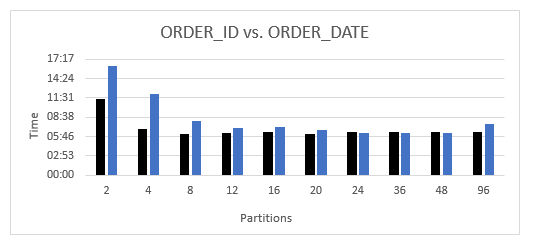
As expected, partitioning with skewed attributes is generally worse than partitioning with uniform attributes. This is especially true of low partition granularities (two, four, or eight partitions). However, when the partitioning reaches sufficient granularity, between 24 and 48 partitions, the effect of the data skew becomes less apparent. The partition granularity is fine enough that the effects of the data skew are masked by the processing overhead of the data extractors.
The obvious conclusion is to use a uniformly distributed attribute as the partitioning column if one is available. You can find a uniform partitioning with near-optimal performance at relatively low granularities, versus the higher granularities needed for a skewed attribute. If a uniform distribution is not available, then a bit more analysis is needed to find an effective partitioning on a skewed attribute.
The alternative approach is to partition the skewed data ranges with sufficient granularity to mitigate the data skew. In our example, this approach would create more partitions in the Q4 timeframe. We compare the two approaches in the following figure.
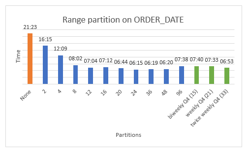
As before, the orange bar (far left) shows the benchmark timing for a migration with no partitioning. The 10 blue bars in the middle of the chart show simple range partitioning with uniform ranges. (This is the same blue bar data shown in the previous figure, ORDER_ID vs. ORDER_DATE.) Lastly, the three green bars show a simple quarterly partitioning for the first nine months of the year, and then a biweekly (once every two weeks), weekly, and twice weekly (once every three or four days) partitioning for the fourth quarter.
The blue bars indicate that the performance impact associated with skewed data can be overcome with uniformly sized partitions if the partition granularity is sufficiently high. You would need to run a set of experiments to find this “sweet spot” (between 24 and 48 partitions in our earlier example). But because the partitioning is uniform, the partition bounds can be easily scripted, which simplifies the discovery process.
The three green bars show the performance for the more “labor intensive” partitioning, which increases the grain of the partitioning over the skewed Q4 data. The performance for this partitioning is essentially equivalent to the uniform partitioning when a sufficient grain is reached. However, creating these partitions requires domain knowledge because you must consider the actual data distributions, identify areas of skew, and adjust the partitioning accordingly.
So, which of the two strategies should you choose? The choice boils down to domain knowledge about the application. If you are familiar with the data and have knowledge about potential data skew, then the second approach is more targeted and can be very effective. Alternatively, if you are not familiar with the data distributions, then trying a series of uniform partition ranges can help you “zero-in” on a near-optimal partitioning with minimal effort. In any case, choosing some partitioning is always better than no partitioning.
Methodology
We can summarize our observations in the following best practices.
- If you have a small number of distinct values or need to filter the source data, use list partitioning.
- If you are using range partitioning, do the following, if possible:
- Choose attributes with uniform distributions.
- Use auto split partitioning.
- If you are forced to use an attribute with a skewed distribution, do the following:
- Test various partition granularities for performance from small to big. You might find close to optimal performance at a fairly small granularity.
- Otherwise, apply domain knowledge to create finer grain partitions on the skewed data.
- In any case, resist the temptation to over-partition because it might not yield sufficient performance gain to offset the required analysis.
Conclusion
We developed the AWS SCT data extractors to automate many of the tasks that you will encounter in migrating your data warehouse to the AWS Cloud. In this blog post, we described how to use virtual partitioning, an AWS SCT best practice for data warehouse migrations. You should use virtual partitions to speed up the migration of large un-partitioned source tables. We looked at the specific types of virtual partitioning supported by AWS SCT, when to use them, and the performance implications for the most common use cases.
Every migration is unique because of your business rules and practices, technical environment, and available personnel and resources. So, you can use the guidelines in this post to inform your migration planning. However, your particular use case will dictate how best to apply virtual partitioning to your migration. Good luck, and happy migrating!
About the Author
 Michael Soo is a database engineer with the AWS DMS and AWS SCT team at Amazon Web Services.