AWS HPC Blog
Running 20k simulations in 3 days to accelerate early stage drug discovery with AWS Batch
This post contributed by Christian Kniep, Sr. Developer Advocate for HPC and AWS Batch at AWS, Carsten Kutzner, staff scientist at the Max Planck Institute for Biophysical Chemistry, and Vytautas Gapsys, project group leader at the Max Planck Institute for Biophysical Chemistry in Göttingen.
Early stage drug discovery helps to identify compounds and optimize them to further develop new drugs within pharmaceutical research. What used to be a slow and exclusively manual discovery process involving laborious chemical synthesis is now accelerated by Computer Aided Drug Design (CADD). In the past, a technique called molecular docking was most widely used. While it’s fast, molecular docking is less accurate compared to molecular dynamics (MD) simulations, where the dynamics of the protein-ligand interaction is simulated explicitly in atomic detail. That accuracy makes CADD a viable and scalable option.
In this blog post, we’ll describe how early stage drug discovery can be accelerated while also optimizing the cost using two popular open-source packages running at scale on AWS. We used GROMACS, which does a molecular dynamics simulations, and pmx, a free-energy calculation package from the Computational Biomolecular Dynamics Group at Max Planck Institute in Germany.
Accelerating early-stage drug discovery with CADD
For each of the tens of thousands of potential compounds in the MD-based drug discovery process, simulations help select candidates for the next pre-clinical development stage. This later stage is much more costly, and therefore only a few hundred compounds can be tested. Applying selection criteria in the initial discovery phases is key for focusing on the right candidates for the later clinical development stage which focuses on only a handful of compounds.

Figure 1: Stages of the drug development process.
Historically, early stage simulations were performed on static on-premises shared compute infrastructure. Today, more research institutions are looking to the AWS Cloud for a scalable alternative that is both cost effective and provides faster turn-around times for getting results.
Optimizing for cost and runtime
In collaboration with the team from Max Planck, we ran an ensemble of twenty thousand molecular dynamics simulations evaluating free energies for drug-like compounds binding to the target proteins. We achieved this in 3 days using an innovative setup to leverage several AWS Regions at once. Using multiple AWS Regions produced a result that was both low cost, but also fast. Optimizing both these variables is important if we’re to cure disease faster.
Instance selection through generic benchmarks
On-premises HPC compute environments tend to be homogenous with respect to the CPU and GPU resources for each node. They also tend to leverage the highest-end CPUs and multiple GPUs at the time of procurement to pack as much compute in the data center as possible.
In AWS, though, there’s a much larger selection of instance types (over four hundred, currently) all optimized to fit different use-cases. With our ensemble run comprising ~20k jobs, it is not the performance of an individual simulation that needs to be maximized. Instead, we aim to minimize the time-to-result to run the complete ensemble while keeping the costs as small as possible. To identify which AWS instances offer a good price-to-performance ratio with GROMACS, the team from Max Planck tested dozens of different instance types using a set of benchmark simulation systems.
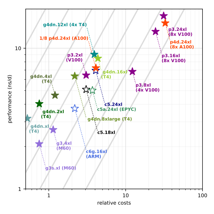
Figure 2: GROMACS 2020 performance as a function of instance costs for the benchmark on CPU (open symbols) and GPU instances (filled symbols). The grey lines show equal performance/price, with better choices to the upper left. Source: “GROMACS in the Cloud: From traditional HPC to global parallelism”.
The data showed that the “usual” high-performance CPU or GPU instances were actually not the best choice for a single simulation. That’s because GROMACS achieves its best performance with a particular ratio of CPU and GPU cores. The analysis showed that the graphics-optimized G4dn instance family ranks highest in performance-to-price. For a deeper dive into our single-node benchmarking, please visit the blog post Running GROMACS on GPU instances: single-node price-performance.
Benchmarking the protein-ligand systems used in the drug discovery ensemble
These initial benchmarks informed the next step in planning the simulation within the first stage of the development of a new drug: simulating the protein-ligand interactions of compounds and estimating their binding free energy.
In the complete ensemble we simulated eight protein-ligand complexes to derive a total of 1,656 free energy differences. Each involved a total of 12 simulations – forward and backward transition of three replicas considering two ligand environments – solvated in water and bound to the protein’s active site. In total, this meant running 19,872 simulations.
The table below shows a comparison of different instance types running the biggest system in the simulation, ‘shp2’ with 107k atoms.

Figure 3: Runtime and price per free energy difference (Spot Instances at the time of benchmarking) run for a 107k atoms system for a selection of instances.
| p4dn.24xl | g4dn.xl | g4dn.2xl | g4dn.4xl | g4dn.8xl | g4dn.16xl | c5.4xl | c5.24xl | c5a.24xl | |
| $/job OD | $159.6 | $50.4 | $48.0 | $57.6 | $87.6 | $165.6 | $117.0 | $182.4 | $223.2 |
| $/job Spot | $49.8 | $16.8 | $16.2 | $19.2 | $28.2 | $51.6 | $46.2 | $70.8 | $94.8 |
| runtime | 6.1h | 12.9h | 8.5h | 6.6h | 6.0h | 6.0h | 26.4h | 8.0h | 9.6h |
Table 1 shows that GPU instances can achieve a turn-around time for a single run of 6 hours. Due to how the simulation can be split and offloaded to GPUs by the GROMACS version used, the simulation is not able to benefit as much from instances that have multiple GPUs. You can find more about how GROMACS leverages CPUs and GPUs in our earlier post — Running GROMACS on GPU instances.
From that study, we learned that the G4dn instance family has the best price-to-performance ratio. For the binding affinity study, our aim was to strike a balance of time-to-result and cost-efficiency by finding Spot Instances that can finish in less than 10 hours. Given these two constraints — instances with the best price-performance and able to finish processing under 10 hours — we used G4dn.2xlarge, G4dn.4xlarge, and G4dn.8xlarge instances. We also leveraged c5.24xlarge instances for additional capacity, since these had an acceptable price-to-performance and were able to accomplish our simulations in the allotted time.
Optimizing for 20k simulations
Because each job can be executed as an independent container within AWS Batch, we knew we could achieve a high level of parallelism. As each job didn’t require large payloads of data, we were able to lean on the entire AWS global infrastructure to provide the necessary capacity by deploying over 25 Regions and 81 Availability Zones.
To simplify the operations of running so many simulations, we chose to split the runs based on the size of the system.
In line with best practices for Spot Instances, we included multiple instance types (g4dn.2xlarge up to g4dn.8xlarge, as well as c5.24xlarge instances for additional capacity) to our compute environments and let the scheduler pick from multiple capacity pools and maximize our usage in a Region, even though that implied somewhat higher cost per job.
Specifically, we ran the large systems on more than 3,500 GPU instances and 1,000 CPU instances across 6 Regions on one day. The next day we ran the small- and medium-sized systems on 4,500 CPU instances, and any remaining systems on CPU instances the third day. You can see the capacity curves in Figure 4, Figure 5, and Figure 6.

Figure 4: Instance count over the course of the ensemble run.

Figure 5: Instance types count over the course of the ensemble run.

Figure 6: Job count over the course of the ensemble run.
Results
For our binding affinity study, we completed 20,000 jobs over the course of three days. By using benchmarks and choosing optimal Spot Instances, we were able to achieve a cost as low as $16 per free energy difference (∆∆G value). As we chose to broaden the set of instances for a shorter time-to-solution, we achieved an average of $40/∆∆G value.
With AWS Batch, we were able to create pools of resources in different AWS Regions around the globe and handle orchestration within the region. By the end of this, it was clear that we could achieve both a really fast wall-clock time (and hence time-to-result) as well as a low overall cost.
Conclusion
In this iteration, we focused on meeting a time-to-result goal. We limited the complexity of this proof of concept by only choosing 6 AWS Regions. We also took a fairly simple approach to instance selection, to get the job finished against a deadline. Our next experiment will be to optimize for cost by picking the Spot Instances to target a $16/∆∆G value, which will likely result in a longer time-to-result.
Further Reading
If you want to try out GROMACS on AWS Batch, visit the GROMACS on AWS ParallelCluster workshop. The workshop will show how GROMACS can be installed and build a container using Spack, a package manager. You can then use that container to run GROMACS on AWS Batch in the Running GROMACS on AWS Batch workshop. Finally, to find out more about AWS Batch, visit our website and documentation.
Some of the content and opinions in this blog are those of the third-party author and AWS is not responsible for the content or accuracy of this blog.