This post summarizes a recent research paper from the AWS Center for Quantum Computing. The paper provides an improved analysis of quantum simulation of chemical and material systems. This research shows that such simulations can be implemented using fewer elementary quantum operations than previously thought.

Computer simulations enable scientists to test their intuition about the properties of physical systems. Simulation results can be compared to experiments for validation. However, if sufficiently accurate simulation methods are available, scientists can test their predictions without having to resort to experiments, which are time consuming and expensive. Current classical simulation methods are not sufficiently accurate when applied to ‘strongly correlated’ systems. This makes it hard for researchers to simulate many systems of practical interest, including high temperature superconductors, photovoltaic materials, and transition metal-based catalysts.

In contrast, quantum algorithms have been developed that can simulate these systems exactly, using resources that scale polynomially with the size of the system. We require an error-corrected quantum computer to run these algorithms. Such a device is still in active development, but will one day be used to solve customer problems that need accurate solutions. This could include assisting in the design of novel materials or compounds, without having to synthesize all of the candidate systems.

It is important to optimize the number of qubits and gates required to implement these algorithms, so that their benefits can be brought to customers, in a shorter timeframe. In this post and the accompanying paper, we dive deep into our new method to calculate the resources required for chemistry and materials simulations. We exploit information about the number of particles in the system, which is not possible using previous techniques. Our approach produces more accurate resource estimates for homogeneous electron gas systems, which enable the calculations to run over 10x faster than prior estimates. We apply our method to systems that are twice as large as is possible using existing methods. This blog post is intended for a technical audience with an undergraduate level understanding of quantum mechanics.

Quantum simulations on quantum computers

When simulating a chemical system, the first step is to find its lowest-lying energy levels, as these will determine many of its properties at room temperature. As a further simplification, we normally model chemical systems as a collection of electrons, which interact with each other in the presence of the electric fields generated by stationary nuclei. Our model then consists of a set of ‘spin orbitals’, into which the electrons are excited by interactions with the other electrons, or with the nuclei. Even these simple models can be very hard to solve. As the electrons can exist in a superposition of different spin orbitals, we could place a system with η electrons and N spin orbitals into a superposition of C(N, η) = ^N! ⁄ _η!(N-η)! (the binomial coefficient N choose η) states – which grows very quickly with both η and N.

Although it can be resource intensive for classical computers to store a large superposition of states, performing this task is natural for quantum computers. By mapping the occupancy of spin orbitals to qubits (we place a qubit in state |1〉 if there is an electron in the spin-orbital, and in state |0〉 if there is not), we can use quantum computers to store and measure states that describe chemical systems. This mapping also lets us write down the ‘Hamiltonian’ (an operator, which measures the energy of the model) of the chemical system, in terms of actions performed on the qubits.

Measuring ground state energies

We will assume that we have the ground state of our model stored on a quantum computer. We denote this state as |Ψ〉. How can we measure the energy of this state? Because the ground state is an eigenstate of the system Hamiltonian, Ĥ , we have that

Ĥ|Ψ〉 = E|Ψ〉

where E denotes the ground state energy. As a result, if we were to evolve the ground state in time, we would simply pick up a global phase:

e^iĤt|Ψ〉 = e^iEt|Ψ〉.

We can measure this phase (and thus, the energy of the state) using an interferometer-based approach. In this approach, one branch of the wave function is time evolved, and the other is not, which builds up a measurable relative phase difference between the branches. This is the main principle underlying the quantum phase estimation algorithm.

As discussed earlier, our mapping enables us to write the Hamiltonian, Ĥ , in terms of qubit operators. However, we do not know how to perfectly express the time evolution operator, e^iĤt , in terms of operations on the qubits. All known decompositions only approximate the time evolution operator up to an error, which we denote by ε . One such method to approximate the time evolution operator is known as ‘Trotterization’. We will assume that we can write the Hamiltonian as the sum of two parts Ĥ = K̂ + V̂  (for example, dividing the Hamiltonian into a kinetic term and a potential term, as occurs in a plane wave basis), and that we can exactly implement e^iK̂t and e^iV̂t on the quantum computer. We can then approximate the time evolution operator by dividing it into a number of small steps of size Δt, and implementing each step as

e^iĤΔt ≈ e^iK̂Δt e^iV̂Δt .

This approximation (known as a 1st order product formula) is exact if K̂ and V̂ commute with each other. However, if they do not commute, the error in each step is proportional to the commutator of K̂  and V̂

ε ∝ |K̂V̂ – V̂K̂| × Δt²

where |…| denotes taking a suitable norm of the operator. Recent work has shown that it can be beneficial to constrain the error estimate to the physical η-electron subspace. This ‘fermionic seminorm’ is smaller than the unrestricted operator norm. However, previous methods of estimating the Trotter error cannot take advantage of electron number information in this way.

We can also define higher-order product formulae, which use different sequences of time evolution under K̂  and V̂  to improve the dependence of the error on Δt. We can make the error smaller by increasing the number of steps used. However, increasing the number of steps used also increases the number of quantum gates required, which slows down the computation. If we can avoid over-estimating the error, we can use the available quantum hardware in the most economical fashion.

Tighter Trotter error bounds

If the kinetic term K̂  is composed of N_K  terms, and the potential term V̂  is composed of N_V  terms, the resulting error operator will be the sum of N_K × N_V  commutators. Each of these commutators must be evaluated and stored in memory, to obtain the tightest bounds. If we use a higher-order product formula, then we have to calculate nested commutators, which further increases the memory and time cost of the calculation.

In our recent paper, we introduce a more accurate and less computationally costly method of calculating the Trotter error bound. Our method works by splitting individual terms into a number of subterms. We then re-group different subterms into groups known as ‘free-fermion Hamiltonians’. We refer to this as ‘factorizing’ the Hamiltonian. A cartoon of this process is shown in figure 1.

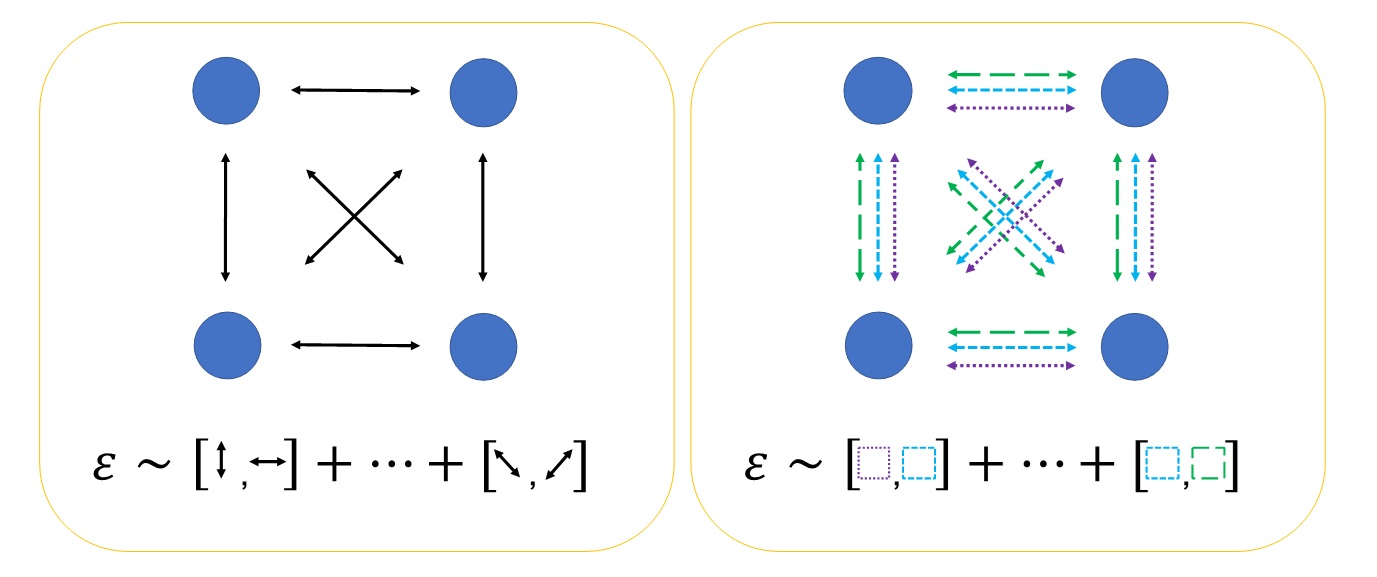
Figure 1: A cartoon illustrating the basis of our improved analysis of Trotter error. In both diagrams, circles represent the spin orbitals of the problem, and the arrows represent interactions between the spin orbitals. The left-hand figure illustrates the existing method for estimating Trotter errors. The error operator is given by the commutators of the different interactions in the Hamiltonian. The right-hand figure illustrates our new method for calculating the Trotter error. Each of the existing interactions is split into a number of terms. These terms are grouped (shown here by the different colors and line styles) into free-fermion Hamiltonians. The error operator is given by the commutators of the free-fermion Hamiltonians, which themselves are free-fermion operators.

We use two key properties of free-fermion Hamiltonians. First, the commutator of two free-fermion Hamiltonians is another free-fermion Hamiltonian. Second, we can efficiently calculate the fermionic seminorm of a free-fermion Hamiltonian. This enables our method to exploit electron number information, which was not possible in previous approaches.

Using these properties, we derive formulas for the Trotter error expressed in terms of the fermionic seminorms of the constituent free-fermion Hamiltonians. We introduce three factorized decompositions – ‘cosine’, ‘cholesky’ and ‘spectral’ – each with their own benefits. For example, our ‘cosine’ decomposition performs best in the low-filling regime. In contrast, our ‘cholesky’ decomposition is most effective when there are half as many electrons as spin orbitals. By introducing three efficient-to-calculate error bounds, we are able to obtain tight resource estimates for many different filling fractions – unlike previous methods.

Reducing resource costs for quantum simulations of chemical systems

We apply our method to calculate the resources required to determine the ground state energy of the homogeneous electron gas. This system is of scientific interest as a simplified model of stellar interiors or fusion experiments. The ground state energy of the homogeneous electron gas is also used to parametrize the models used in density functional theory (the most widely used method to simulate chemistry on classical computers).

We first show how our new bounds are able to exploit electron number information. We calculate the Trotter error bounds for a second-order product formula, for a 2D homogeneous electron gas system discretized with 200 spin orbitals. We plot the scaling of the Trotter error bounds in figure 2. All of our new bounds outperform the existing method in the low filling fraction regime, which is relevant for high accuracy calculations. In addition, our ‘cholesky’ decomposition bound outperforms the existing method in the half-filling regime, relevant for qualitative calculations.

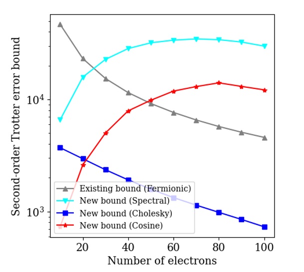
Figure 2: Trotter error bound scaling for second-order Trotter, for a 2D homogeneous electron gas system discretized with 200 spin orbitals, as a function of the number of electrons in the system. The ‘spectral’, ‘cosine’, and ‘cholesky’ decompositions are introduced in this work, while the ‘Fermionic’ bound is the existing method.

We can use our new Trotter error bound estimates in existing compilations of the quantum phase estimation algorithm to determine the number of quantum gates required to calculate the ground state energy of the homogeneous electron gas. We compare the resource costs obtained with our methods, to those obtained with previous Trotter error estimation methods. As shown in Table 1, our improved Trotter error bounds result in tighter resource estimates than previous approaches. The gate count is reduced by a factor of approximately 13, compared to the previous method of costing Trotter-based phase estimation.

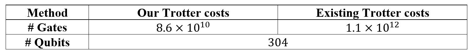
Table 1: The number of elementary gates and logical qubits required for performing quantum phase estimation on a homogeneous electron gas system. The 2D homogeneous electron gas system has 10 electrons in 288 spin orbitals. The number of logical qubits is given by the sum of the 288 qubits representing the spin orbitals, and the 16 additional qubits required to realise the chosen algorithm. Our improved Trotter error bounds reduce the gate count of Trotter-based phase estimation by a factor of ~13.

In the accompanying paper, we also compare our Trotter-based method against an alternative approach known as ‘qubitization’. Qubitization is more involved than Trotter-based approaches, and requires additional ancilla qubits. We find that our Trotter-based approach scales more favorably when the electron density in the system is low, while qubitization scales best in the high-density regime. By improving Trotter error estimates, our work ensures that quantum hardware can be used in the most economical way, at low, intermediate, and high densities.

Conclusion

In this blog post, we have outlined our new method for obtaining more accurate resource estimates for Trotter-based quantum simulations. Our technique is applicable to much larger system sizes than is possible using existing methods, and can exploit electron number information. By introducing three efficient-to-calculate error bounds, we can ensure that we use the tightest available error bounds in all parameter regimes. This means we can provide customers the most resource-efficient algorithm for their problem; whether they wish to study the warm, dense matter inside stars, or precisely determine the phase diagram of the dilute electron gas.

To find out more about our work in quantum simulation algorithms, you can read our paper here, or our closely related work estimating the resources to simulate the Fermi-Hubbard model, a prototypical model of superconductivity. For discussions of how these algorithms can be implemented on error-corrected hardware, see our papers on lattice surgery or our architecture blueprint.

If you’d like to join the quantum computing group at AWS, check out our open jobs. We’re hiring in research science, software, algorithms, and hardware development. And if you want to use currently available quantum computers for your own research in quantum algorithms and hardware, check out Amazon Braket and the AWS Cloud Credit for Research program.