AWS Quantum Technologies Blog
Optimization with a Rydberg atom-based quantum processor
Amazon Braket recently launched the Aquila quantum processing unit (QPU) based on Rydberg atoms by QuEra Computing. In a previous post, we explored how researchers can use Rydberg devices to study problems and quantum phenomena in fundamental physics, for instance the emergence of a spin liquid phase [Semeghini et al., 2021]. But QuEra’s device also enables researchers to study quantum algorithms in new regimes. In this post, we review a recent publication, “Quantum optimization of maximum independent set using Rydberg atom arrays” [Ebadi et al., Science (2022)], in which the authors report the largest deployment of a variational algorithm to date, used to solve combinatorial optimization problems on a Rydberg device similar to the one launched on Nov 1 on Amazon Braket.
In the publication [Ebadi et al., Science (2022)], researchers from Harvard University, in collaboration with scientists from QuEra Computing, MIT, and the University of Innsbruck, reported on using Rydberg atom-based quantum processors to compute solutions for a particular graph coloring problem: finding the maximum independent set (MIS), which is relevant for optimal resource allocation, for example. By running a quantum-classical hybrid algorithm on the device, researchers were able to find the MIS for a class of graphs with a probability that scales favorably with the difficulty of the problem when compared to a classical simulated annealing approach. This work not only highlights the potential of Rydberg-atom devices for solving hard optimization problems, but also opens new research directions.
Maximum independent set
First, let us look at what an MIS problem really is. Edges between nodes of a graph may represent a wide variety of relationships, e.g., social ties between people, railroad connections between cities, or wiring between electrical components. Many optimization problems can be simplified to a task of coloring (or labeling) graph nodes while respecting certain rules.
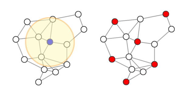
Figure 1. Left: In a unit-disk graph, edges are created between nodes that are closer to each other than a certain fixed distance on the 2-d plane. Right: Red nodes mark a MIS of the graph corresponding to the largest number of nodes (six) that are not directly connected. [source: Ebadi et al., Science (2022)]
Finding an MIS is related to other computational tasks on graphs (e.g., finding cliques and dominant sets), and can be extended to sampling or enumerating all MISs of a graph. Many optimization problems in finance, bioinformatics, logistics, and automation can be mapped to such tasks [Wurtz et al., (2022)].
Discovering an MIS is a computationally hard problem even for the class of 2-d unit-disk graphs (Pichler et al., (2018)) and deciding whether an MIS of a certain size exists for such a graph is NP-complete. The running time of an exhaustive search increases exponentially with the size of the graph. Promising approaches to this include the “branch and bound” algorithm, which guarantees the best solutions but has exponential complexity in the worst case. This means that while these approaches may be fast for easy problem instances, for the hardest graphs (where the number of almost maximal independent sets is much larger than the number true MISs) they still take exponentially long to arrive at the solution. Another approach is to use heuristic algorithms, such as simulated annealing, which can compute independent sets quickly even for large graphs (with a few thousand nodes), and these provide good-enough practical solutions to many use cases, but these methods provide no guarantees that the result is actually an MIS. In particular, the chance of arriving at an MIS also decreases with the difficulty of the problem. Quantifying this difficulty for heuristic algorithms is one of the main achievements of this work. Another achievement of this work is showing that quantum effects can improve the algorithms’ likelihood of success.
Computing the maximum independent set with Rydberg atoms
Rydberg-atom quantum computers, like QuEra’s Aquila device on Amazon Braket, are well suited to study quantum algorithms for MIS problems on unit disk graphs. By arranging the individual atom using optical tweezers, the graph can be directly encoded in the atom positions with each graph node represented by an atom.
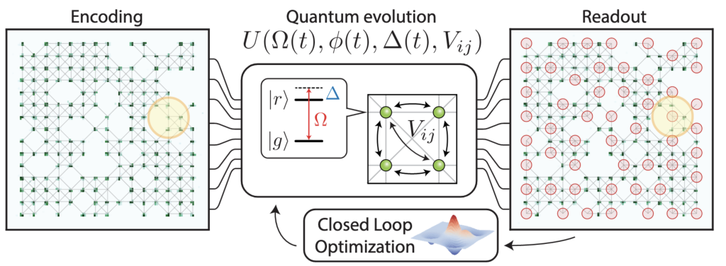
Figure 2. Left: Atoms (green spots) are arranged in a 2-d plane to realize a unit disk graph, where nodes are connected by an edge if they are closer than the Rydberg blockade radius (yellow circle). Middle: A coherent driving field with time-dependent amplitude and detuning is used to steer the evolution of the system from a non-excited state to a maximally excited state constrained by Rydberg blockade () between nearby atoms. Right: An image of the final state is captured with an optical microscope. Missing spots (red circles) mark the locations of excited atoms, the collection of which corresponds to the discovered MIS of the graph. A classical optimizer is used to enhance the probability of finding an MIS. [source: Ebadi et al., Science (2022)]
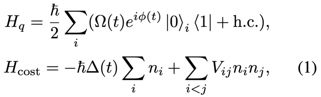
Equation 1. The driving Hamiltonian induces coherent mixing between ground and Rydberg states of all atoms . The time-dependent driving amplitude is ramped up from zero to high values at the beginning of the evolution and ramped down to zero at the end (See Figure 3, red curve). This mixing ensures that the cost of the joint state of all atoms stays low even as the cost Hamiltonian is gradually changed by slowly increasing the detuning parameter from negative to positive values (See Figure 3, blue curve).
Here the driving Hamiltonian transitions the atoms between ground states and excited states for searching an MIS. The pairwise Rydberg interactions , however, prevents neighboring atoms from both being excited if their distance is within a certain range. Hence, this Rydberg “blockade” interaction naturally implements the rule that nodes connected by an edge cannot both be part of an independent set, and its range is illustrated with a yellow circle on Figure 2. To find an MIS, a high reward for Rydberg excitations is added to the objective Hamiltonian , which favors solutions with the highest number of red nodes. Throughout the evolution, the system remains in the approximate instantaneous ground state of the Hamiltonian. At the end of the evolution, the driving Hamiltonian is turned off, and an image of the final state is taken with an optical microscope, from which the value of is computed.
An MIS of the graph corresponds to an atomic configuration with the lowest . To enhance the probability of finding an MIS, the evolution is repeated multiple times, to estimate the average across shots, followed by using a classical optimizer to update the parameters of the quantum evolution. This variational optimization method continually updates the parameters of driving amplitude the detuning, until convergence where is minimized.
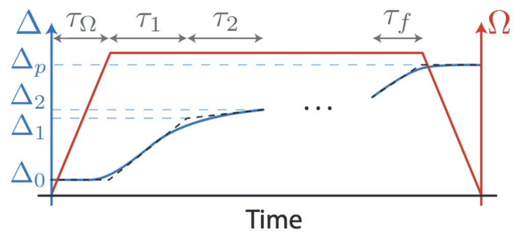
Figure 3. The schedule of the amplitude and the detuning of the driving field for the variational quantum adiabatic algorithm. The amplitude is a constant, except the ramping periods, and the smoothened piecewise-linear time series of the detuning parameter are optimized with a closed-loop optimization. [source: Ebadi et al., Science (2022)]
Comparison with simulated annealing
In Ebadi et al., Science (2022), the authors tested different parametrizations of the schedules and found that the variational quantum adiabatic algorithm (VQAA, shown in Figure 3) can find the MIS with higher probability than the quantum approximate optimization algorithm (QAOA, where the detuning is kept at zero and the driving phase is changed in a stepwise fashion). They also compared VQAA to its classical counterpart, namely the simulated annealing algorithm. This algorithm works by simulating the thermal jitter of a fictitious mechanical system whose energy landscape matches the cost function in question. Throughout the algorithm, the temperature parameter is gradually decreased, causing the system to relax to low-energy states, thereby discovering the local optima of the cost function.
The authors found that the probability of finding an MIS for either VQAA or simulated annealing depends on the “hardness” of the graph. Intuitively, if the graph supports many MISs, it is easy for both algorithms to find an MIS; conversely, if the graph has only few MISs compared to a large number of sub-optimal independent sets with one less node , then both algorithms struggle. The authors compared the probability with which the MIS is returned by the two methods for a range of graphs and for a fixed number of steps that both algorithms are allowed to perform. For some of the hardest graphs, with up to 80 nodes, they found that VQAA was able to approach the MIS in fewer steps, while simulated annealing remained stuck in local minima with fewer red nodes. For a particularly hard case, the quantum algorithm produced the correct MIS with 10 times higher probability than simulated annealing. To quantify the expected advantage of the VQAA on the quantum device over simulated annealing, the authors compared how is decreasing with increasing hardness for the two algorithms: VQAA exhibited a more favorable scaling (with an exponent of -0.63) compared to simulated annealing (which scaled with an exponent of -1.03). The difference amounts to a superlinear improvement of success probability PMIS.
The probability of finding an MIS with the quantum algorithm was found to crucially depend on the minimal spectral gap: the smaller the energy difference between the two lowest energy states, the slower the adiabatic transition needs to be to guarantee a high probability of finding an MIS. Yet, if time evolution is too slow, decoherence and atom loss limits the performance. Specifically, the paper finds that the required time scales polynomially with the inverse of the minimum gap; the dependence of the gap size with problem size and specific instance is unknown. Still, this is an optimistic result; as technology evolves and coherence times improves, the ensemble of MIS problems for which these quantum processors offer an improved performance compared to simulated annealing is expected to increase.
Solving MIS with Rydberg simulator on Amazon Braket
Let us now take a look how we can put these ideas into action. In this section we will demonstrate how to create the graph from Figure 2, and solve the corresponding unit disc problem with Aquila on Braket. Using the Braket python SDK, the following code can be used to define the analog Hamiltonian simulation program that realizes an MIS search on a fixed unit disk graph with a fixed schedule and run it on QuEra’s Aquila QPU.
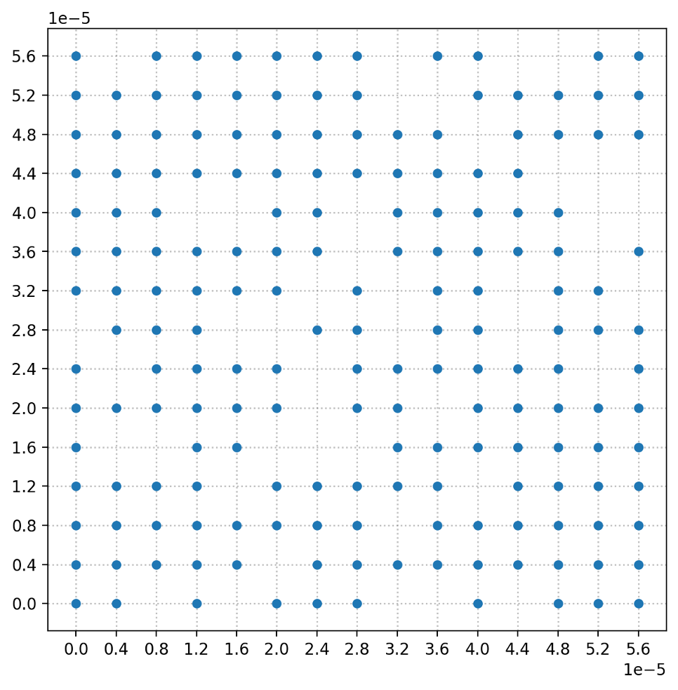
First, we define the atom arrangement that realizes the unit disk graph defined by our optimization problem. Later, we are going to program the time-dependent parameters so that they realize a blockade radius of about 6 micrometers, which means placing the atoms in a square grid with lattice spacing of 4 microns realizes the unit disk graph shown in Figure 2.
To visually confirm the correctness of the register, we plot its atomic positions with the following code:
Next, we define the time-dependent parameters of the Hamiltonian, the amplitude, detuning, and phase of the driving field, to realize a simple adiabatic transition sequence.
Finally, we combine the atom array object and the Hamiltonian into an analog Hamiltonian simulation program and run it on QuEra’s Aquila QPU for 100 shots.
Once the status of the task is COMPLETED (which can be checked with task.metadata()["status"], or on the tasks page of the Braket console), we can query the results withresult = task.result()
The result.measurements object contains a list of shot results. The list, measurements[shot_idx].pre_sequence may contain “0”s which mark sites where atom preparation failed (hence unintentionally missing atoms), and “1”s everywhere else. The measurements[shot_idx].post_sequence measurement results indicate the states of the atoms (“0” for Rydberg state, “1” for ground state) in each of the shot_idx in range(300) shots, where the sequence of atoms is identical to the sequence in which they were added to register, earlier. Shot results containing the most Rydberg stats are the QPU’s best estimates for solving the MIS problem, as they represent the Rydberg atoms, which correspond to the red nodes.
Note, we only run one half iteration of the VQAA optimization algorithm, as we did not adjust the time series parameters of the AHS program. To go beyond this, you can use Amazon Braket Hybrid jobs feature to evolve the system iteratively to minimize the cost function and find the optimal MIS.
Conclusion
The work by Ebadi et al. (Ebadi et al., Science (2022)) realizes a quantum variational optimization algorithm that achieves superlinear improvement compared to classically simulated annealing. Despite the exciting results, many open questions remain. It is unclear for even larger graphs how well VQAA can converge and if the superlinear scaling improvement is retained. Further investigations are needed to compare VQAA’s performance with other state-of-the-art classical approaches, and study how to find the MIS for non-unit-disc graphs on Rydberg systems [Nguyen et al., (2022)].
Our goal is to enable researchers in industry and academia to investigate these questions. With the launch of QuEra’s Aquila QPU to Amazon Braket, a global community of researchers is now able to access state-of-the-art Rydberg computing technology on demand and over the cloud, to advance the understanding of quantum algorithms.
To get started with using the QuEra QPU on Amazon Braket, refer to our AHS example notebooks. For more information about pricing, refer to our Pricing Page. Researchers from accredited institutions can apply for credits by submitting a research proposal here.