Accelerate your data warehouse migration to Amazon Redshift – Part 6

This is the sixth in a series of posts. We’re excited to share dozens of new features to automate your schema conversion; preserve your investment in existing scripts, reports, and applications; accelerate query performance; and potentially simplify your migrations from legacy data warehouses to Amazon Redshift.

Amazon Redshift is the cloud data warehouse of choice for tens of thousands of customers who use it to analyze exabytes of data to gain business insights. With Amazon Redshift, you can query data across your data warehouse, operational data stores, and data lake using standard SQL. You can also integrate other AWS services such as Amazon EMR, Amazon Athena, Amazon SageMaker, AWS Glue, AWS Lake Formation, and Amazon Kinesis to use all the analytic capabilities in the AWS Cloud.

Migrating a data warehouse can be a complex undertaking. Your legacy workload might rely on proprietary features that aren’t directly supported by a modern data warehouse like Amazon Redshift. For example, some data warehouses enforce primary key constraints, making a tradeoff with DML performance. Amazon Redshift lets you define a primary key but uses the constraint for query optimization purposes only. If you use Amazon Redshift, or are migrating to Amazon Redshift, you may need a mechanism to check that primary key constraints are not being violated by extract, transform, and load (ETL) processes.

In this post, we describe two design patterns that you can use to accomplish this efficiently. We also show you how to use the AWS Schema Conversion Tool (AWS SCT) to automatically apply the design patterns to your SQL code.

We start by defining the semantics to address. Then we describe the design patterns and analyze their performance. We conclude by showing you how AWS SCT can automatically convert your code to enforce primary keys.

Primary keys

A primary key (PK) is a set of attributes such that no two rows can have the same value in the PK. For example, the following Teradata table has a two-attribute primary key (emp_id, div_id). Presumably, employee IDs are unique only within divisions.

CREATE TABLE testschema.emp ( 
  emp_id INTEGER NOT NULL
, name VARCHAR(12) NOT NULL
, div_id INTEGER NOT NULL
, job_title VARCHAR(12)
, salary DECIMAL(8,2)
, birthdate DATE NOT NULL ) 
CONSTRAINT pk_emp_id PRIMARY KEY (emp_id, div_id);

Most databases require that a primary key satisfy two criteria:

• Uniqueness – The PK values are unique over all rows in the table
• Not NULL – The PK attributes don’t accept NULL values

In this post, we focus on how to support the preceding primary key semantics. We describe two design patterns that you can use to develop SQL applications that respect primary keys in Amazon Redshift. Our focus is on INSERT-SELECT statements. Customers have told us that INSERT-SELECT operations comprise over 50% of the DML workload against tables with unique constraints. We briefly provide some guidance for other DML statements later in the post.

INSERT-SELECT

In the rest of this post, we dive deep into design patterns for INSERT-SELECT statements. We’re concerned with statements of the following form:

INSERT INTO <target table> SELECT * FROM <staging table>

The schema of the staging table is identical to the target table on a column-by-column basis.

A duplicate PK value can be introduced by two scenarios:

• The staging table contains duplicates, meaning there are two or more rows in the staging data with the same PK value
• There is a row x in the staging table and a row y in the target table that share the same PK value

Note that these situations are independent. It can be the case that the staging table contains duplicates, the staging table and target table share a duplicate, or both.

It’s imperative that the staging table doesn’t contain duplicate PK values. To ensure this, you can apply deduplication logic, as described in this post, to the staging table when it’s loaded. Alternatively, if your upstream source can guarantee that duplicates have been eliminated before delivery, you can eliminate this step.

Join

The first design pattern simply joins the staging and target tables. If any rows are returned, then the staging and target tables share a primary key value.

Suppose we have staging and target tables defined as the following:

CREATE TABLE stg ( 
  pk_col INTEGER 
, payload VARCHAR(100) 
, PRIMARY KEY (pk_col)
); 

CREATE TABLE tgt ( 
  pk_col INTEGER 
, payload VARCHAR(100) 
, PRIMARY KEY (pk_col)
);

SELECT count(1) 
FROM stg, tgt 
WHERE tgt.pk_col = stg.pk_col;

If the primary key has multiple columns, then the WHERE condition can be extended:

SELECT count(1)
FROM stg, tgt
WHERE
    tgt.pk_col1 = stg.pk_col1
AND tgt.pk_col2 = tgt.pk_col2
AND …
;

There is one complication with this design pattern. If you allow NULL values in the primary key column, then you need to add special code to handle the NULL to NULL matching:

SELECT count(1)
FROM stg, tgt
WHERE
   (tgt.pk_col = stg.pk_col) 
OR (tgt.pk_col IS NULL AND stg.pk_col IS NULL)
;

This is the primary disadvantage of this design pattern—the code can be ugly and unintuitive. Furthermore, if you have a multicolumn primary key, then the code becomes even more complicated.

INTERSECT

The second design pattern that we describe uses the Amazon Redshift INTERSECT operation. INTERSECT is a set-based operation that determines if two queries have any rows in common. You can check out UNION, INTERSECT, and EXCEPT in the Amazon Redshift documentation for more information.

We can determine if the staging and target table have duplicate PK values using the following query:

SELECT COUNT(1)
FROM (
  SELECT pk_col FROM stg
  INTERSECT
  SELECT pk_col FROM tgt
) a
;

If the primary key is composed of more than one column, you can simply modify the subqueries to include the additional columns:

SELECT COUNT(1)
FROM (
  SELECT pk_col1, pk_col2, …, pk_coln FROM stg
  INTERSECT
  SELECT pk_col, pk_col2, …, pk_coln FROM tgt
) a
;

This pattern’s main advantage is its simplicity. The code is easier to understand and validate than the join design pattern. INTERSECT handles the NULL to NULL matching implicitly so you don’t have to write any special code for NULL values.

Performance

We tested both design patterns using an Amazon Redshift cluster consisting of 12 ra3.4xlarge nodes. Each node contained 12 CPU and 96 GB of memory.

We created the staging and target tables with the same distribution and sort keys to minimize data redistribution at query time.

We generated the test data artificially using a custom program. The target dataset contained 1 billion rows of data. We ran 10 trials of both algorithms using staging datasets that ranged from 20–200 million rows, in 20-million-row increments.

In the following graph, the join design pattern is shown as a blue line. The intersect design pattern is shown as an orange line.

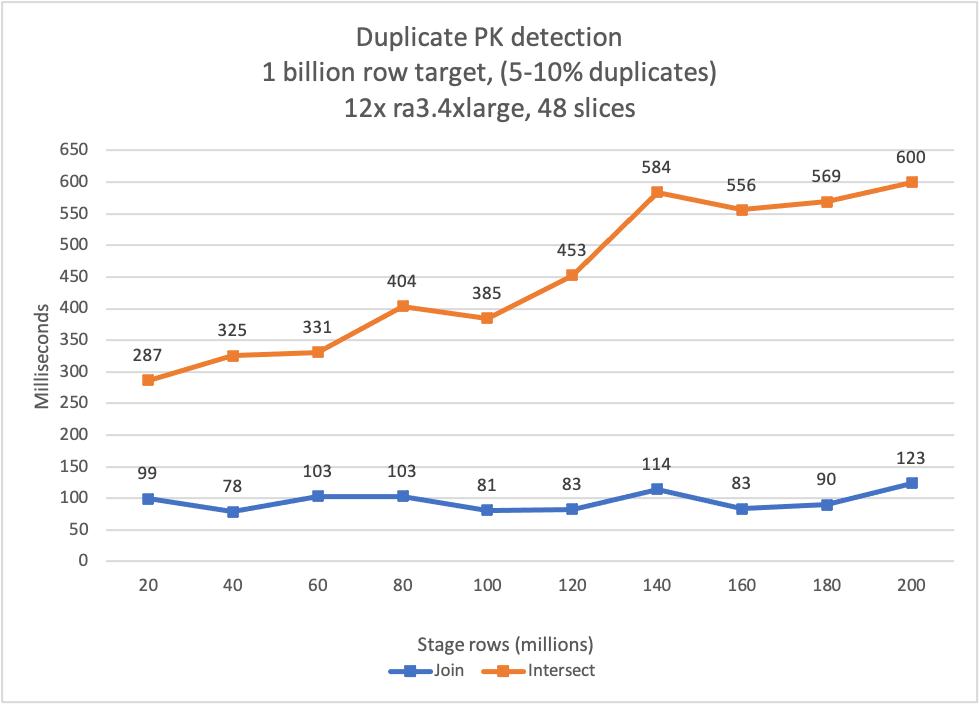
You can observe that the performance of both algorithms is excellent. Each is able to detect duplicates in less than 1 second for all trials. The join algorithm outperforms the intersect algorithm, but both have excellent performance.

So, which algorithm should use you choose? If you’re developing a new application on Amazon Redshift, the intersect algorithm is probably the best choice. The inherent NULL matching logic and simple intuitive code make this the best choice for new applications.

Conversely, if you need to squeeze every bit of performance from your application, then the join algorithm is your best option. In this case, you’ll have to trade complexity and perhaps extra effort in code review to gain the extra performance.

Automation

If you’re migrating an existing application to Amazon Redshift, you can use AWS SCT to automatically convert your SQL code.

Let’s see how this works. Suppose you have the following Teradata table. We use it as the target table in an INSERT-SELECT operation.

CREATE MULTISET TABLE testschema.test_pk_tgt (
  pk_col INTEGER NOT NULL
, payload VARCHAR(100) NOT NULL
, PRIMARY KEY (pk_col)
);

The staging table is identical to the target table, with the same columns and data types.

Next, we create a procedure to load the target table from the staging table. The procedure contains a single INSERT-SELECT statement:

REPLACE PROCEDURE testschema.insert_select()
BEGIN
INSERT INTO testschema.test_pk_tgt (pk_col, payload)
SELECT pk_col, payload FROM testschema.test_pk_stg;
END;

Now we use AWS SCT to convert the Teradata stored procedure to Amazon Redshift. First, open Settings, Conversion settings, and ensure that you’ve selected the option Automate Primary key / Unique constraint. If you don’t select this option, AWS SCT won’t add the PK check to the converted code.

Next, choose the stored procedure in the source database tree, right-click, and choose Convert schema.

AWS SCT converts the stored procedure (and embedded INSERT-SELECT) using the join rewrite pattern. Because AWS SCT performs the conversion for you, it uses the join rewrite pattern to leverage its performance advantage.

And that’s it, it’s that simple. If you’re migrating from Oracle or Teradata, you can use AWS SCT to convert your INSERT-SELECT statements now. We’ll be adding support for additional data warehouse engines soon.

In this post, we focused on INSERT-SELECT statements, but we’re also happy to report that AWS SCT can enforce primary key constraints for INSERT-VALUE and UPDATE statements. AWS SCT injects the appropriate SELECT statement into your code to determine if the INSERT-VALUE or UPDATE will create duplicate primary key values. Download the latest version of AWS SCT and give it a try!

Conclusion

In this post, we showed you how to enforce primary keys in Amazon Redshift. If you’re implementing a new application in Amazon Redshift, you can use the design patterns in this post to enforce the constraints as part of your ETL stream.

Also, if you’re migrating from an Oracle or Teradata database, you can use AWS SCT to automatically convert your SQL to Amazon Redshift. AWS SCT will inject additional code into your SQL stream to enforce your unique key constraints, and thereby insulate your application code from any related changes.

We’re happy to share these updates to help you in your data warehouse migration projects. In the meantime, you can learn more about Amazon Redshift and AWS SCT. Happy migrating!

About the authors

Michael Soo is a Principal Database Engineer with the AWS Database Migration Service team. He builds products and services that help customers migrate their database workloads to the AWS cloud.

Illia Kravtsov is a Database Developer with the AWS Project Delta Migration team. He has 10+ years experience in data warehouse development with Teradata and other MPP databases.