Accelerate HNSW indexing and searching with pgvector on Amazon Aurora PostgreSQL-compatible edition and Amazon RDS for PostgreSQL

It’s important to understand strategies for how to use pgvector with your Generative AI applications so you can find the optimal configurations. This can include the selection of your database instance family, how you ingest your data, and even the version of pgvector you’re using.

We ran a series of tests to see how pgvector 0.5.1 performed compared to the previous version (0.5.0), and workload characteristics on Graviton2 and Graviton3 instances on Amazon Aurora PostgreSQL-compatible edition and Amazon RDS for PostgreSQL. We used the HNSW (hierarchical navigable small worlds) index method in pgvector for this test. For the workloads we tested, we observed that pgvector 0.5.1 can ingest vectors up to 225% faster than pgvector 0.5.0, and for searching over vectors with high dimensionality (1536 dimensions) with higher concurrency (64 clients), Graviton3 instances can outperform Graviton2 by 60%.

In this post, we explore several strategies to help maximize performance when using HNSW indexing with pgvector on and Amazon Relational Database Service (Amazon RDS) for PostgreSQL.

Background: Using pgvector for Retrieval Augmented Generation (RAG)

Generative AI applications can use a technique called Retrieval Augmented Generation (RAG) that provides additional context to foundational models to provide domain-specific results to users. A key component of RAG is a vector data store, which provides an efficient storage and retrieval mechanism to recall information that can be used by a foundational model to provide an enhanced answer. To prepare a vector data store for RAG, you must first convert raw data, such as text documents, by passing it through an embedding model, such as Amazon Titan, and turning them into a set of corresponding vectors that provide a mathematical representation of the data. From there, users of a generative AI application can perform actions such as ask questions, and the application can perform a vector similarity search to find the best solution to augment the foundational model. The following graphic demonstrates the ingestion and retrieval workflow used in RAG.

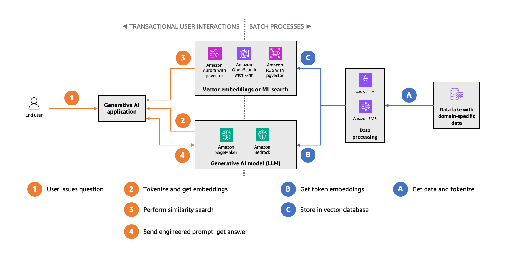
In the ingestion workflow, raw data from a source such as a data lake (A) is converted by batch processes into vectors of tokens (B) and stored in a vector database (C). During transactional user interactions, the user issues a question (1), which is converted into vectors of tokens (2) and presented to the vector database for a similarity search (3). The result of the database query is merged with the tokenized user question to generate a richer prompt for better answers from the generative AI model (4).

pgvector is an open-source extension available for Amazon Aurora PostgreSQL-Compatible Edition and Amazon RDS for PostgreSQL that adds vector database capabilities, including a vector data type, distance operations, and several indexing methods. One aspect of successfully using pgvector in your Generative AI application is choosing and configuring the appropriate index method. The next section provides an overview of how indexing works with pgvector.

Understanding approximate nearest neighbor indexing

Finding similar vectors, also known as nearest neighbor or K-NN queries, can be a time-consuming process. This is because a query must compare the distance of every single vector in a dataset to find the top candidates. Although searching over every vector in a dataset provides the best quality results, a generative AI application may be able to trade off result quality for speed.

Approximate nearest neighbor (ANN) algorithms can help accelerate these searches by searching over a subset of vectors in the dataset, though this can impact the quality of results. The metric used to measure result quality is recall, which measures the percentage of expected results for a given query. ANN algorithms provide tuning parameters that let you choose the performance/recall trade-off that’s appropriate for your application.

The pgvector extension provides two ANN index methods: IVFFLAT and, as of 0.5.0, HNSW (hierarchical navigable small worlds). HNSW is a graph-based indexing method that groups similar vectors into increasingly dense layers, which allows for efficient, high-quality searches over a smaller set of vectors. Both Amazon Aurora and Amazon RDS support HNSW indexing with pgvector. Amazon RDS for PostgreSQL recently added pgvector 0.5.1 to version 15.4-R3, which contains performance improvements for high-concurrency workloads that require HNSW indexing.

Let’s explore how pgvector works so we can build strategies to use it to effectively index and search data in our application.

Prerequisites

For the experiment, we used RDS for PostgreSQL instances, specifically with version 15.4-R3, and pgvector 0.5.1. These experiments can also be run with Amazon Aurora PostgreSQL-compatible edition. The experiment compared pgvector 0.5.1 to using 0.5.0. Additionally, for the purposes of benchmarking, we used a db.m7g.16xlarge instance and a db.m6g.16xlarge instance, both with default configurations, and used gp3 storage with 20,000 provisioned IOPS. For the client instance, we used an Amazon Elastic Compute Cloud (Amazon EC2) c6in.8xlarge instance that is positioned in the same Availability Zone as the databases (for example, us-east-2a).

About the testing methodology

When reviewing the performance of a vector data store, particularly when using an ANN search, it’s important to evaluate four characteristics:

• Performance – How fast does a query return a result?
• Recall – What is the quality of the results?
• Build time – How long does it take to build an index?
• Size – How much storage does the data require?

These characteristics are used both by vector data store designers and users to understand how well a data store works for vector workloads. This post focuses primarily on query performance and index build time. We don’t focus on size because the vector storage size is either fixed or not important to the outcome of the tests demonstrated in this post.

Although it’s essential to consider recall when building an application that uses an ANN method such as HNSW, we address recall indirectly in this post when we discuss query performance with the hnsw.ef_search parameter. Higher values of hnsw.ef_search typically provide better recall. Additionally, you can often improve recall by increasing the index construction parameters m and ef_construction, but the strategies outlined in this post are applicable regardless of these values. This post uses the default values for m and ef_construction provided in pgvector 0.5.1, which are m=16 and ef_construction=64.

Data ingestion with pgvector and HNSW on Amazon RDS for PostgreSQL

The first step to setting up an RDS for PostgreSQL database for RAG workflows is to prepare it to store vectors. In this section, we show how concurrent inserts, or inserting vectors from different clients, can help accelerate building an HNSW index in pgvector. As of version 0.5.1, pgvector doesn’t support parallel index builds for HNSW, but concurrent inserts offer a way to speed up index build times. HNSW is an iterative algorithm, which means that you can continue to add vectors to the HNSW index over time. This makes it possible to use the concurrent insertion method.

To run this example, you must first ensure pgvector is installed in your PostgreSQL database. You can install pgvector in your database by running the following command:

CREATE EXTENSION IF NOT EXISTS vector;

You will see the following output:

CREATE EXTENSION

For our ingestion test, we want to generate random vectors. The following PL/pgSQL takes an argument of dim and generates a normalized vector that has dim dimensions:

CREATE OR REPLACE FUNCTION generate_random_normalized_vector(dim integer)
RETURNS vector
LANGUAGE plpgsql
AS $$
DECLARE
    a real[];
    mag real;
    x real;
    i int;
BEGIN
    SELECT array_agg(random()::real) INTO a FROM generate_series(1, dim);

    mag := public.vector_norm(a::vector);

    FOR i IN 1..dim
    LOOP
        a[i] := a[i] / mag;
    END LOOP;

    RETURN a::vector;
END;
$$;

You will see the following output:

CREATE FUNCTION

For testing ingestion performance, we use the pgbench PostgreSQL utility. pgbench is a benchmarking tool that comes with PostgreSQL. You can provide your own custom benchmarking scripts for pgbench. For this data ingestion test, we created a script that inserts a randomly generated dimensions into a table called vecs. Create a file called pgvector-hnsw-concurrent-insert.sql and add the following code:

\setshell vector_dim echo ${VECTOR_DIM:-128}

INSERT INTO vecs (embedding)
SELECT public.generate_random_normalized_vector(':vector_dim');

This script uses a pgbench command, \setshell, to pass in an arbitrary value for the vector dimension, defaulting to 128 dimensions. Note that generating the random vector can take 0.5 to 2 milliseconds, which has a marginal impact on ingestion performance, but we opt for this method due to convenience.

We now have enough to set up the ingestion test. For this test, we see how many vectors we can insert into each environment over a period of 15 minutes (900 seconds). Running the test for a prolonged period of time helps normalize the effects of other operations on the server, client, and network. For each iteration of the test, we increase the number of clients, and use a ratio of one client per job, where a job is equivalent to one thread. Also, between each test run, we must drop any previously created index, remove all the data from the table, and create an empty index.

We use the following commands to run the ingestion test:

export PGHOST="<database host>"
export PGUSER="<database user>"
export PGPASSWORD="<database password>"
export PGDATABASE="<database name>"
export VECTOR_DIM=128
TEST_TIME=900
VECTOR_OPS="vector_l2_ops"
for clients in 1 2 4 8 16 32 64; do
    psql -c "DROP INDEX IF EXISTS vecs_embedding_idx;"
    psql -c "TRUNCATE TABLE vecs;"
    psql -c "CREATE INDEX ON vecs USING hnsw(embedding ${VECTOR_OPS});"
    pgbench -n -T "${TEST_TIME}" \
      --file=pgvector-hnsw-concurrent-insert.sql \
      -c "${clients}" -j "${clients}"
done

As the test runs, you’ll see output similar to the following:

pgbench (16.0 (Ubuntu 16.0-1.pgdg22.04+1), server 15.4)
transaction type: pgvector-hnsw-concurrent-insert.sql
scaling factor: 1
query mode: simple
number of clients: 64
number of threads: 64
maximum number of tries: 1
duration: 900 s
number of transactions actually processed: 8127088
number of failed transactions: 0 (0.000%)
latency average = 7.081 ms
initial connection time = 870.289 ms
tps = 9038.789025 (without initial connection time)

For the first run, we inserted 128 dimensional vectors into a table. The table was created using the following SQL:

CREATE TABLE vecs (
    id int GENERATED BY DEFAULT AS IDENTITY,
    embedding vector(128)
);

You will see the following output:

CREATE TABLE

The following table shows the results of the different runs. As mentioned earlier, these tests were performed using gp3 storage with 20,000 provisioned IOPS and used the Euclidean (L2) distance operation and measured using transactions per second (TPS):

Let’s look more closely at these results. In these experiments, we can observe two factors that impacted ingestion times:

• Using pgvector 0.5.0 and 0.5.1
• The instance type used

The first test kept the instance type fixed (db.m7g.16xlarge) but used two different version of pgvector (0.5.0 and 0.5.1). As the number of clients increases, we can see that pgvector 0.5.1 can index vectors more rapidly than 0.5.0. With 64 clients concurrently inserting vectors, pgvector 0.5.1 showed a 225%, or 3.25 times, speedup over pgvector 0.5.0.

The following table shows the results presented in the above chart:

The bulk of this speedup comes from two pull requests (refer to Speed up HNSW index build and Improve HNSW index build performance more) in pgvector that reduce the number of distance calculations performed when inserting elements.

The second test kept the version of pgvector fixed (0.5.1) but used two different instance types (db.m7g.16xlarge, db.m6g.16xlarge). In this test run, we observe that there is a general performance increase in using the m7g family of instances.

The following table shows the results presented in the above chart:

The m7g instance family uses the Graviton3 processor, which contains general performance improvements and specific improvements targeted for floating point calculations. Vector workloads using pgvector can benefit from the newer Graviton processors to help accelerate workloads, as these tests show.

The preceding tests use a 128-dimensional vector, but many embedding models use larger vectors. For example, Amazon Titan embeddings generate a 1,536-dimensional vector to represent its embeddings. We can repeat the earlier test to determine how pgvector and Amazon RDS for PostgreSQL work with a 1,536-dimensional vector. To set up the test, first recreate the vecs table to store a 1,536-dimensional vector:

DROP TABLE IF EXISTS vecs;
CREATE TABLE vecs (
    id int GENERATED BY DEFAULT AS IDENTITY,
    embedding vector(1536)
);

You can now run the tests for vectors with 1,536 dimensions. You can use the same script as before, but change VECTOR_DIM to be 1536:

export PGHOST="<database host>"
export PGUSER="<database user>"
export PGPASSWORD="<database password>"
export PGDATABASE="<database name>"
export VECTOR_DIM=1536
TEST_TIME=900
VECTOR_OPS="vector_l2_ops"
for clients in 1 2 4 8 16 32 64; do
    psql -c "DROP INDEX IF EXISTS vecs_embedding_idx;"
    psql -c "TRUNCATE TABLE vecs;"
    psql -c "CREATE INDEX ON vecs USING hnsw(embedding ${VECTOR_OPS});"
    pgbench -n -T "${TEST_TIME}" \
      --file=pgvector-hnsw-concurrent-insert.sql \
      -c "${clients}" -j "${clients}"
done

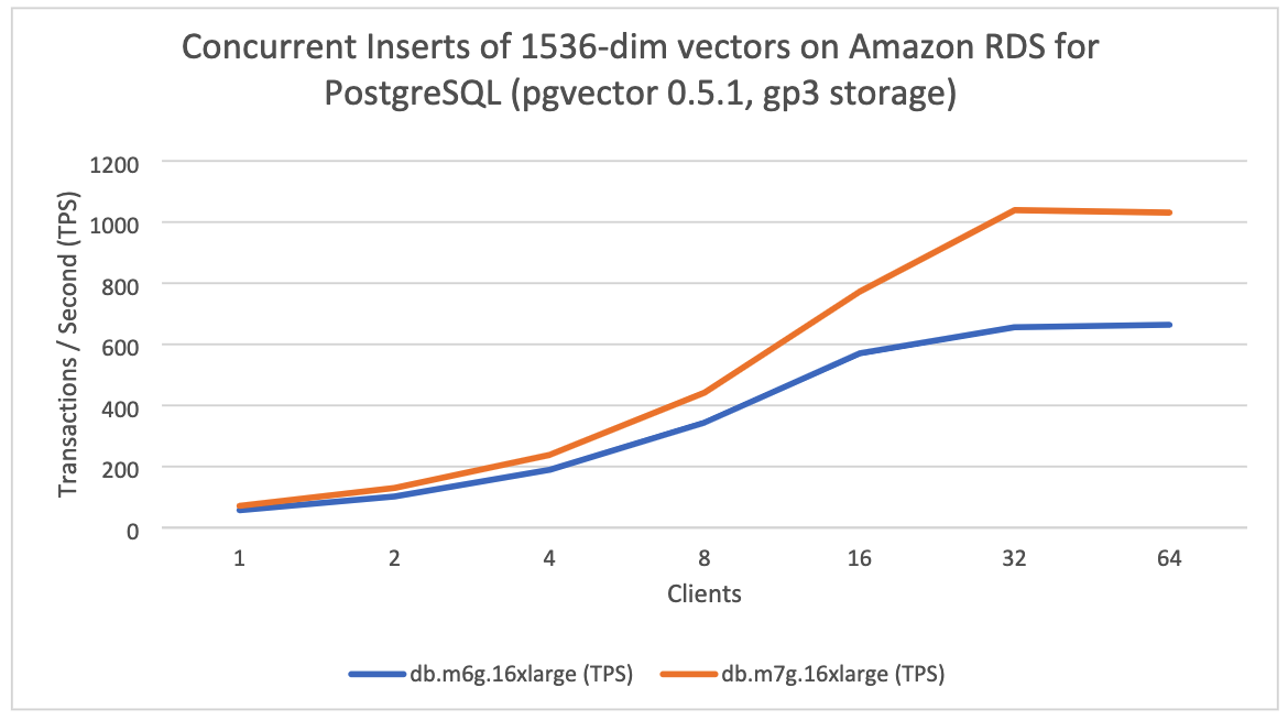
The following table shows the results of the different runs with the 1,536-dimensional vector dataset. As mentioned earlier, these tests were performed using gp3 storage with 20,000 provisioned IOPS and used the Euclidean (L2) distance operation and measured using transactions per second (TPS).

For the first test, where we varied pgvector versions (0.5.0, 0.5.1), we observed a speedup but not as significant as on the 128-dimensional vector dataset. You can see the results in the following figure:

The following table shows the results presented in the above chart:

The speedup in the test with the 1,536-dimensional vectors is not as large as the 128-dimensional vectors primarily due to how the vectors are stored. The fundamental storage unit in PostgreSQL is called a page, which can store up to 8 KB of data. A 128-dimensional vector requires about 0.5 KB of storage, whereas a 1,536-dimensional vector requires about 6 KB. Therefore, a 1,536-dimensional vector will take up an entire page, whereas you can fit multiple 128-dimensional vectors on the same page. When building an HNSW index, pgvector will need to read more pages to index a 1,536-dimensional vector compared to a 128-dimensional vector, which can take additional time if the pages aren’t in active memory. The improvements in pgvector 0.5.1 target reducing the number of calculations, so although the 1,536-dimensional vectors do benefit from them, you may observe less benefit over smaller vectors due to the amount of space the larger vectors require.

For the second test, where we varied the instance class (db.m6g.16xlarge, db.m7g.16xlarge), we observed a larger speedup particularly as the number of clients increased. You can see the results in the following figure:

The following table shows the results presented in the above chart:

As mentioned previously, Graviton3 processors contain optimizations that can help accelerate floating point calculations. It takes additional effort to calculate the distance between 1,536-dimensional vectors due to their size, which means the m7g instance family can accelerate processing these vectors.

Now that we’ve observed how pgvector 0.5.1 contains performance improvements on index building and how your choice of instance type can affect ingestion performance, let’s review how these decisions impact query performance.

Query performance with pgvector and HNSW on Amazon RDS for PostgreSQL

One reason HNSW is a popular choice for vector queries is due to its general performance while achieving high recall. In the previous section, we observed that instance type could impact HNSW index build times. But what effect does instance selection have on query performance on this dataset?

For this test, we use pgvector 0.5.1 and only vary the instance type (db.m6g.16xlarge, db.m7g.16xlarge). Like the previous test, we use gp3 storage with 20,000 provisioned IOPS. For each run, all of the vectors in the dataset were indexed and the table and vector data were loaded into memory.

This test used a process-based multiprocessor written in Python to run queries. Each process generated 50,000 random normalized vectors, connected to the database, and simultaneously ran queries. We used this to calculate the total number of queries processed per second. To simulate recall levels, we performed this test with increasing values of hnsw.ef_search. Each test run measured performance by calculating the number of transactions run per second (TPS).

The following results used a dataset of 10,000,000 128-dimensional vectors. The table used 5.45 GB of storage, and the HNSW index used 7.75 GB of storage.

Overall, for the 128-dimensional dataset, the query performance results were comparable between the db.m6g.16xlarge and the db.m7g.16xlarge. However, we observed that the query performance on the db.m7g.16xlarge was consistently around 10% faster with 64 clients on higher values of hnsw.ef_search.

We repeated the experiment using 10,000,000 1,536-dimensional vectors, which have the same dimensions as the vectors generated by the Amazon Titan embeddings. The table used 39 GB of storage, and the index used 38 GB of storage. We ran a similar experiment, where we compared the query performance with different values of hnsw.ef_search with 64 clients concurrently executing queries. As with the earlier experiment, we compared the db.m6g.16xlarge and db.m7g.16xlarge instances. You can see the results in the following figure:

The following table shows the results presented in the above chart:

Overall, for the 1,536-dimensional dataset, the db.m7g.16xlarge instance generally outperformed the d6.m6g.16xlarge instance by 10%. However, we saw a notable increase in performance for 64 clients, particularly as we increased hnsw.ef_search, the parameter that helps influence recall. We observed that the db.m7g.16xlarge had a 40–60% speedup over the db.m6g.16xlarge for querying 1,536-dimensional vectors, because we can use the improvements in the m7g instance family that help workloads that are CPU heavy perform better.

Clean up

If you ran these tests on your own Amazon Aurora or RDS for PostgreSQL and EC2 instances, and don’t require the instances for any additional tasks, then you can delete the instances.

Conclusion

In this post, we walked through different methods that you can use to accelerate ingestion and query performance when using the HNSW indexing functionality in pgvector on Amazon Aurora PostgreSQL-compatible edition and Amazon RDS for PostgreSQL. We also observed how performance improvements in pgvector 0.5.1 can speed up concurrent ingestion, and how new instance classes can accelerate queries.

Understanding methods to optimize your usage of a vector index such as HNSW can make a difference in both your ingestion and query performance. These strategies can help you optimize your database configuration and design your applications so that you can take full advantage of the index functionality. You can use the techniques in this post to help you start building your generative AI applications with pgvector on Amazon Aurora PostgreSQL-compatible edition and Amazon RDS for PostgreSQL!

We invite you to leave feedback in the comments.

About the author

Jonathan Katz is a Principal Product Manager – Technical on the Amazon RDS team and is based in New York. He is a Core Team member of the open source PostgreSQL project and an active open source contributor.f