Build a real-time fraud detection solution using Amazon Neptune ML

Each year online businesses lose tens of billions of dollars due to fraud, which can take many forms. For example, fraudsters can obtain stolen credit card details and use them for unauthorized transactions. Therefore, detecting fraud and malicious behavior at the time of a transaction, such as when a user registers a new payment method, is necessary for working to prevent these fraud-related losses. The following diagram shows a fraud detection use case where a business predicts if a purchase request using a credit card is fraudulent or not based on data on known fraud.

In this post, we demonstrate how you can build a real-time fraud detection solution using Amazon Neptune ML. With Neptune ML, and in particular the real-time inductive inference capability, we can build solutions for businesses to provide real-time alerts regarding fraudulent transactions to help reduce their fraud loss and increase revenue.

With real-time inductive inference for Amazon Neptune ML, Neptune customers can get near real-time predictions on new data by using existing Neptune ML models without retraining their ML models each time. Additionally, they can train and deploy Neptune ML models faster and save costs by training on a representative sample of their graph data, and then deploying it to make predictions on any entity in the graph.

Machine learning (ML) based methods learn from data to create models that can robustly identify different fraud patterns and techniques that fraudsters use to mask their behavior and evade detection, at scale. Recently, a class of ML models called graph neural networks (GNN) has emerged as a powerful method for fraud detection. GNNs are trained on a graph representation of the interconnecting data, and they outperform traditional ML approaches that don’t directly utilize the connections between entities present in the graph.

Amazon Neptune is a fast, reliable, and fully-managed graph database service that makes it simple to build and run applications that work with highly connected datasets. Neptune ML is a feature of Neptune that enables users to automate the creation, management, and usage of GNN ML models using the graph data stored in Neptune. Neptune ML is built using Amazon SageMaker and Deep Graph Library, and it provides a simple and convenient mechanism for customers with graph data to build/train/maintain these models. Then, they can use the predictive capabilities of these models within a Gremlin or SPARQL query to predict elements or property values in the graph.

With the release of Neptune version 1.2.0.2, Neptune ML supports real-time inductive inference, which applies data processing and model evaluation in real-time on new data. Previously, you needed to run an offline processor to process and compute predictions for new nodes or edges added to the graph database after training. However, with real-time inductive inference, you can get model predictions with graph queries as soon as new data is added to the database.

Solution overview

Building a real-time fraud detection solution with Neptune ML requires the following key components:

1. The Fraud Graph Data Model – You must collect and transform your data into a graph data model in a format that you can load into Neptune.
2. Machine Learning Task – You must formulate the fraud detection problem as a graph ML task that can be solved by Neptune ML.
3. Machine Learning Workflow – You must follow the Neptune ML workflow to export the graph data, train the GNN model, and create the model inference endpoints.
4. Making Predictions – Once the ML model is deployed to an inference endpoint, you can use graph queries to make the predictions on data that was originally in the graph, as well as newly added data.

We demonstrate a solution using the IEEE CIS dataset, a dataset with anonymized real-world e-commerce transactions, and perform fraud detection using node classification, one of the ML tasks supported by Neptune ML. With node classification, a model is learned for predicting a property of the nodes in a graph where values of the node property already observed are used as training examples to train another model which can then predict that property for other nodes in the graph. Specifically, the type of node classification task to be demonstrated here is a binary classification. The property we’re trying to predict is the isFraud property, which denotes whether or not the node is an instance of fraudulent transactions. Although many ML approaches can be used to tackle this problem, GNN models like those provided by Neptune ML are unique because they directly utilize both the graph structure and node properties to make predictions.

Prerequisites

To build this solution, you should have the following prerequisites:

• A Neptune cluster (engine version 1.2.0.2 or later) with Neptune ML configured. The simplest way is to use the AWS CloudFormation quick-start template. This template installs all necessary components, including a new Neptune DB cluster. Typically, it takes 10 minutes to deploy all the resources. You can also install Neptune ML manually on top of an existing Neptune DB cluster, as described in Setting up Neptune ML without using the quick-start AWS CloudFormation template.
• An Amazon Simple Storage Service (Amazon S3) bucket in the same region as the Neptune cluster.
• A Neptune graph notebook instance. The Neptune ML AWS CloudFormation quick-start template includes installing a new Neptune graph notebook. We’ll host our graph notebook using the Neptune workbench, and then use it to illustrate the solution steps. You can find the full notebook used in this post in this GitHub repo.
• You are responsible for the costs incurred when you try this tutorial from your AWS account. There are no additional charges for using Amazon Neptune ML real-time inductive inference. You only pay for the resources provisioned such as Amazon Neptune, Amazon SageMaker, Amazon CloudWatch, and Amazon S3. For more information on pricing and region availability, refer to the Neptune pricing page and AWS Region Table.

The fraud graph data model

To demonstrate our solution, we first use the IEEE CIS dataset to build a fraud graph. In general, a fraud graph stores not only transactional data with basic attribute information, but also relationships between the transactions, actors, what kinds of products are purchased, shared devices, shared addresses, and more. The dataset originally represents the data in tabular form. It contains Transaction and Identity tables, both having many anonymized columns. These also have a Transaction ID as the primary key column. The first task is to convert the tabular data into a graph data model, defining the relationships of the transaction records with cards, devices, products, and other identifiers as shown in the following figure.

Converting that tabular dataset to graph data has been discussed in the previous post, Build a GNN-based real-time fraud detection solution using Amazon SageMaker, Amazon Neptune, and the Deep Graph Library, which used the same dataset. The same basic principle of converting the tabular data to graph data can be applied. In other words, for each pair of columns from the tables, where one is the transaction ID column and the other is a categorical column, two nodes are created using the values of the columns (if not already created), and an edge between the two nodes is created. The values of the columns in the Transaction table become the properties of the transaction nodes.

The results of converting the tabular data into the graph data based on the principle are shown as follows. You get at least four types of nodes and the relationships between them:

To summarize, here are the nodes and edges that we deal with in our graph:

Nodes:

• Transaction: The values of the columns in the Transaction table become the properties of the transaction nodes.
• Device: with properties deviceInfo and deviceType.
• Identifier: with only ID.
• Card: with only ID.

Edges:

• Identified_by: A transaction is identified by multiple identifiers.
• Purchased_by: A transaction is a purchase with a credit card.
• Associated_with: A transaction is associated with a device.

Neptune ML workflow

Amazon Neptune ML provides a simple workflow for training ML models on graph data in Neptune. It uses a four-step workflow to automate the process of creating production-ready GNN models:

• Export Data – A Neptune-export-service call is made specifying the ML model type and model configuration parameters. Then, the data and model configuration parameters are exported from a Neptune cluster to an S3 bucket.
• Data Processing – The exported dataset is preprocessed using standard techniques to prepare for model training.
• Model Training – A set of service calls are made to train the ML model and tune the model hyper parameters, and then generate a SageMaker model that can be deployed to an endpoint that exposes the model.
• Inference endpoint creation – A SageMaker endpoint instance is launched with the model artifacts produced by the best training job.

As shown below, we use the Neptune workbench to illustrate the steps of the Neptune ML workflow. Neptune workbench contains a line magic %neptune_ml and a cell magic %%neptune_ml that can save you a lot of time managing these steps.

Exporting data

The first step is to export the data to Amazon S3 using the Neptune export service. To speed up the export of a graph of considerable size, you can clone a cluster to perform the task of exporting the data. Neptune export service can automatically create a clone of the cluster to complete the data export to Amazon S3. Exporting from the existing cluster requires that the neptune_query_timeout parameter in the parameter group be set to a large enough value (>72000) to prevent timeout errors. To limit the amount of data to be exported, additional parameters, such as nodeLabels and edgeLabels, can be used to explicitly include the nodes and edges to be exported.

export_params={ 
"command": "export-pg", 
"params": { "endpoint": neptune_ml.get_host(),
            "profile": "neptune_ml",
            "useIamAuth": neptune_ml.get_iam(),
            "cloneCluster": True,
             "cloneClusterInstanceType": "r5.12xlarge",
             "nodeLabels": ["Transaction", "Identifier", "Device", "Card"],
             "edgeLabels": ["identified_by", "purchased_by", "associated_with"]
            }, 
"outputS3Path": f'{s3_bucket_uri}/neptune-export',
"additionalParams": {
        "neptune_ml": {
          "version": "v2.0",
          "targets": [
            {
              "node": "Transaction",
              "property": "isFraud",
              "type": "classification"
            }
          ]
        }
      },
"jobSize": "medium"}

%%neptune_ml export start --export-url {neptune_ml.get_export_service_host()} 
--export-iam --wait --store-to export_results ${export_params}

Once the export job is completed, you can train your ML model and create the inference endpoint. Training your Neptune ML model requires three steps.

Data processing

The next step is to process the exported graph dataset in Amazon S3 using standard feature preprocessing techniques to prepare it for use by DGL. For example, the numerical properties are scaled or normalized and the categorical and text properties are encoded to numeric vectors. This step is implemented using a SageMaker Processing Job that runs in your account. The resulting data artifacts are stored in a pre-specified S3 bucket once the job is complete.

# The training_job_name can be set to a unique value, otherwise one will be auto generated
training_job_name=neptune_ml.get_training_job_name('node-classification')
outputS3Uri = export_results['outputS3Uri']

processing_params = f"""
--config-file-name training-data-configuration.json
--job-id {training_job_name} 
--s3-input-uri {outputS3Uri} 
--s3-processed-uri {str(s3_bucket_uri)}/preloading """

%neptune_ml dataprocessing start --wait --store-to processing_results {processing_params}

Model training

The second step trains the ML model that will be used for predictions. The model training has two stages. The first stage uses a SageMaker Processing job to generate a model training strategy which is a configuration set that specifies what type of model and model hyperparameter ranges will be used for the model training. Once this is complete, the SageMaker Processing job launches a SageMaker Hyperparameter tuning job, which runs a pre-specified number of model training job trials on the processed data, and then it stores the model artifacts generated by the training in the output S3 bucket. Once the training jobs are complete, the job also notes the training job that produced the best performing model. In the second stage, the best performing model is applied to the full exported graph dataset to generate the model artifacts for deployment.

training_params=f"""
--job-id {training_job_name} 
--data-processing-id {training_job_name}
--instance-type ml.p3.2xlarge
--s3-output-uri {str(s3_bucket_uri)}/training 
--max-hpo-number 2
--max-hpo-parallel 2 """

%neptune_ml training start --wait --store-to training_results {training_params}

Inference endpoint creation

The final step is to create the inference endpoint, which is a SageMaker endpoint instance that is launched with the model artifacts produced by the best training job. This endpoint will be used for making predictions later on. Once created, the endpoint stays active until it’s manually deleted. Each model is tied to a single endpoint.

endpoint_params=f"""
--id {training_job_name}
--model-training-job-id {training_job_name}"""

%neptune_ml endpoint create --wait --store-to endpoint_results {endpoint_params}

Model visualization

One way to inspect the ML model is by examining the node embeddings generated as part of the ML artifacts. For node classification tasks, Neptune ML saves the model predictions and node embeddings to the output S3 bucket. For visualization, you can plot the node embeddings in reduced dimensions with the predicted class as a legend. The following plot shows that there is a clear separation between the nodes that represent fraudulent transactions and those that represent legitimate transactions.

Making predictions

Depending on the nature of the business use case, you can make different types of predictions with the Neptune ML model endpoint. If you want to make predictions on data that was already present in the graph at the time of training, but whose property was unknown, then the transductive inference queries are fast and efficient, since the predictions can be precomputed at the end of training. On the other hand, if your graph is dynamic, and you want to make predictions on new data added to the graph after the training process or see how new data affects the model prediction for an existing node, then real-time inductive inference is the best choice.

Transductive inference

During the training process, Neptune ML pre-computes and stores a model prediction for every node in the graph. Then, this can be looked up quickly when queried. This is referred to as “transductive inference”. It requires that the nodes being queried for prediction were in the graph at the time of model training.

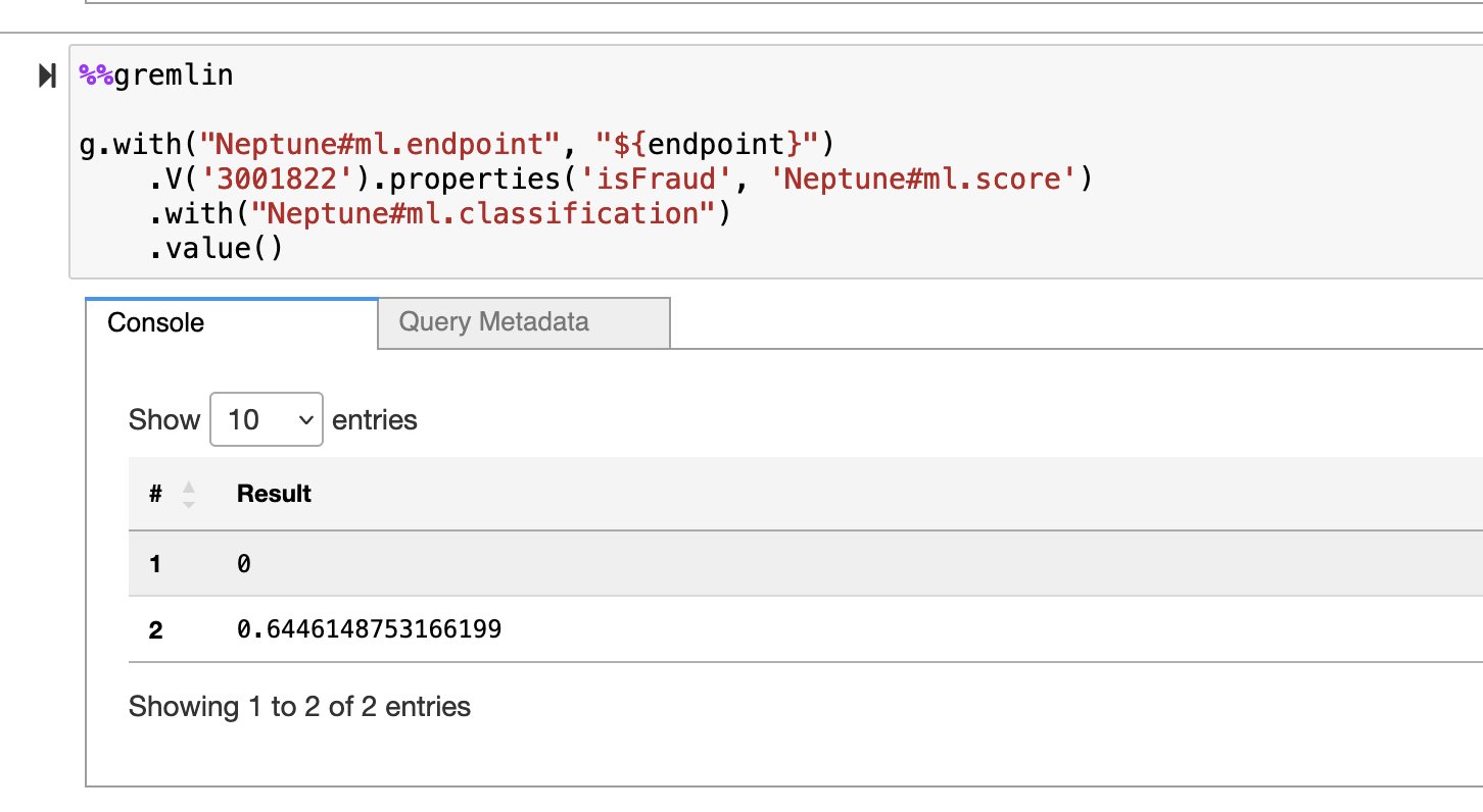
For example, the following Gremlin query retrieving the isFraud property of the transaction with ID 3001822 returns no data:

g.V('3001822').properties("isFraud")

This indicates that the isFraud property is missing. Since this transaction was present in the graph at training time, transductive inference can be used to predict the missing property. To do that, we add two steps in the Gremlin query:

• specify the inference endpoint that we want to use,
• specify the type of ML task.

To the previous query, we add two with() steps to specify the inference endpoint and node classification as the ML task. Running the following query will return the predicted value (either 0 or 1) of the isFraud property for that transaction. It will also return the prediction probability assigned to the predicted label because of the inclusion of Neptune#ml.score.

g.with("Neptune#ml.endpoint", "${endpoint}")
    .V('3001822').properties('isFraud', 'Neptune#ml.score')
    .with("Neptune#ml.classification").value()

This screenshot shows the results of running the transductive inference with the Gremlin query in the notebook.

Instead of predicting one missing property, you can use the following query to make the prediction on the transactions that miss the isFraud property.

g.with("Neptune#ml.endpoint", "${endpoint}")
    .V().hasLabel('Transaction').hasNot("isFraud")
    .properties('isFraud').with("Neptune#ml.classification").value()

Inductive inference

In a real-time application, you must make predictions on new data as it is added to the database. Specifically, in the context of the IEEE-CIS dataset, a new transaction node with edges connecting existing or new nodes may be added. The question is: how likely is it that this new transaction is a fraudulent transaction? Inductive inference can be used here to answer that question.

In real-time inductive inference mode, GNN models can make predictions for newly appeared nodes and edges. To demonstrate that, we first run a query to create a new Transaction node with ID 9999999 and a few edges connecting the new node with a device, a card, and a couple of identifiers. For this demonstration, we use the existing device node with ID DeviceType:mobile, card node with ID card3:150.0, and identifier nodes with IDs id_05:0.0 and id_38:F.

g.addV('Transaction').property(T.id, '9999999')
               .property('id_01', -5.0)
               .property('id_02', 222578.0)
               .property('id_05', 0.0)
               .property('id_06', 0.0)
               .property('id_11', 100.0)
               .property('id_12', 'NotFound')
               .property('id_13', 49.0)
               .property('id_14', -300.0)
               .property('id_15', 'New')
               .property('id_16', 'NotFound').as('newT')
  .addE('associated_with')
               .from('newT')
               .to(V('DeviceType:mobile'))
               .property(T.id, 'transaction_9999999-associated-with-mobile')         
  .addE('purchased_by')
               .from('newT')
               .to(V('card3:150.0'))
               .property(T.id, 'transaction_9999999-purchased-by-card')
  .addE('identified_by')
               .from('newT')
               .to(V('id_05:0.0'))
               .property(T.id, 'transaction_9999999-identified-by-id_05')
  .addE('identified_by')
               .from('newT')
               .to(V('id_38:F'))
               .property(T.id, 'transaction_9999999-identified-by-id_38') 

The following screenshot shows a sub-graph of a transaction node connecting with its neighboring nodes.

The following Gremlin query on the property of the new transaction will return no value. This reflects how the isFraud property is unknown.

g.V('9999999').properties("isFraud").value()

If the cluster is enabled with Real-time Inductive Inference, then you can use a Gremlin query to obtain the predicted value of the isFraud property of the new transaction. The Gremlin query must:

• specify the inference endpoint that we want to use.
• specify the type of ML task.
• specify the type of inference, which is inductiveInference. If the type isn’t specified, then the default is transductive inference. For a new node, no result of inference will be returned.
• specify the type of sampling in the case of inductive inference, which can be either “deterministic” or “non-deterministic”. When using inductive inference, the Neptune engine creates the appropriate subgraph to evaluate the trained GNN model, and the requirements of this subgraph depend on the parameters of the final model.  By default, an inductive inference query builds the neighborhood randomly. When you include Neptune#ml.deterministic in an inductive inference query, the Neptune engine attempts to sample neighbors in a deterministic way so that running the same query returns the same results.

The following query will return a string of either “1” or “0” deterministically, thereby indicating if this transaction is likely fraudulent or not.

g.with("Neptune#ml.endpoint",'${endpoint}')
  .V('9999999').properties("isFraud")
  .with("Neptune#ml.classification")
  .with("Neptune#ml.inductiveInference")
  .with("Neptune#ml.deterministic")
  .value()

It’s possible to combine both the mutation and the inference into one query. This is shown in the following screenshot where the creation of the node and edges and the inductive inference are combined, with Neptune#ml.score specified to obtain the result with the confidence score.

You can change the type of sampling to “non-deterministic” which is the default.

g.with("Neptune#ml.endpoint",'${endpoint}')           
  .V('9999999').properties("isFraud", "Neptune#ml.score")
  .with("Neptune#ml.classification")
  .with("Neptune#ml.inductiveInference")
  .value()

Clean up

When you’re finished exploring the solution, you can run the cell below to delete the inference endpoint to avoid incurring unnecessary charges.

neptune_ml.delete_endpoint(training_job_name)

Conclusion

In this post, we demonstrated how you can use Neptune ML and real-time inductive inference to build a real-time fraud detection solution.  Using a graph data model based on the IEEE-CIS dataset, we walked through the steps of training a ML model, creating an inference endpoint, and performing both transductive and inductive inferences in real-time using the inference endpoint.

To learn more about real-time inductive inference, see the Neptune ML documentation page. Reach out to us if you need help in building your application.

About the Authors

 Hua Shu is a Senior Neptune Specialist Solution Architect at Amazon Web Services. She has over 20 years of experience in software development. Currently she is focusing on working with customers to build graph database-based applications.

Soji Adeshina is an Applied Scientist at Amazon Web Services where he develops graph neural network-based models for machine learning on graphs tasks with applications to fraud & abuse, knowledge graphs, recommender systems, and life sciences. In his spare time, he enjoys reading and cooking.